3.9: Logarithmic Regression - Class Notes
Contents
Thursday, November 21, 2019
Overview
Today, we finish up our view of nonlinear models with logarithmic models, which are more frequently used. We also discuss a few other tests and transformations to wrap up multivariate regression before we turn to panel data: standardizing variables to compare effect sizes, and joint hypothesis tests.
Interpretting logged variables can often be difficult to remember, so here I reproduce the tables that describe the interpretations of the marginal effect of X→Y, as well as some visual examples from the slides:
| Model | Equation | Interpretation |
|---|---|---|
| Linear-Log | Y=β0+β1ln(X) | 1% change in X→^β1100 unit change in Y |
| Log-Linear | ln(Y)=β0+β1X | 1 unit change in X→^β1×100% change in Y |
| Log-Log | ln(Y)=β0+β1ln(X) | 1% change in X→^β1% change in Y |
- Hint: the variable that gets logged changes in percent terms, the variable not logged changes in unit terms
| Linear-Log | Log-Linear | Log-Log |
|---|---|---|
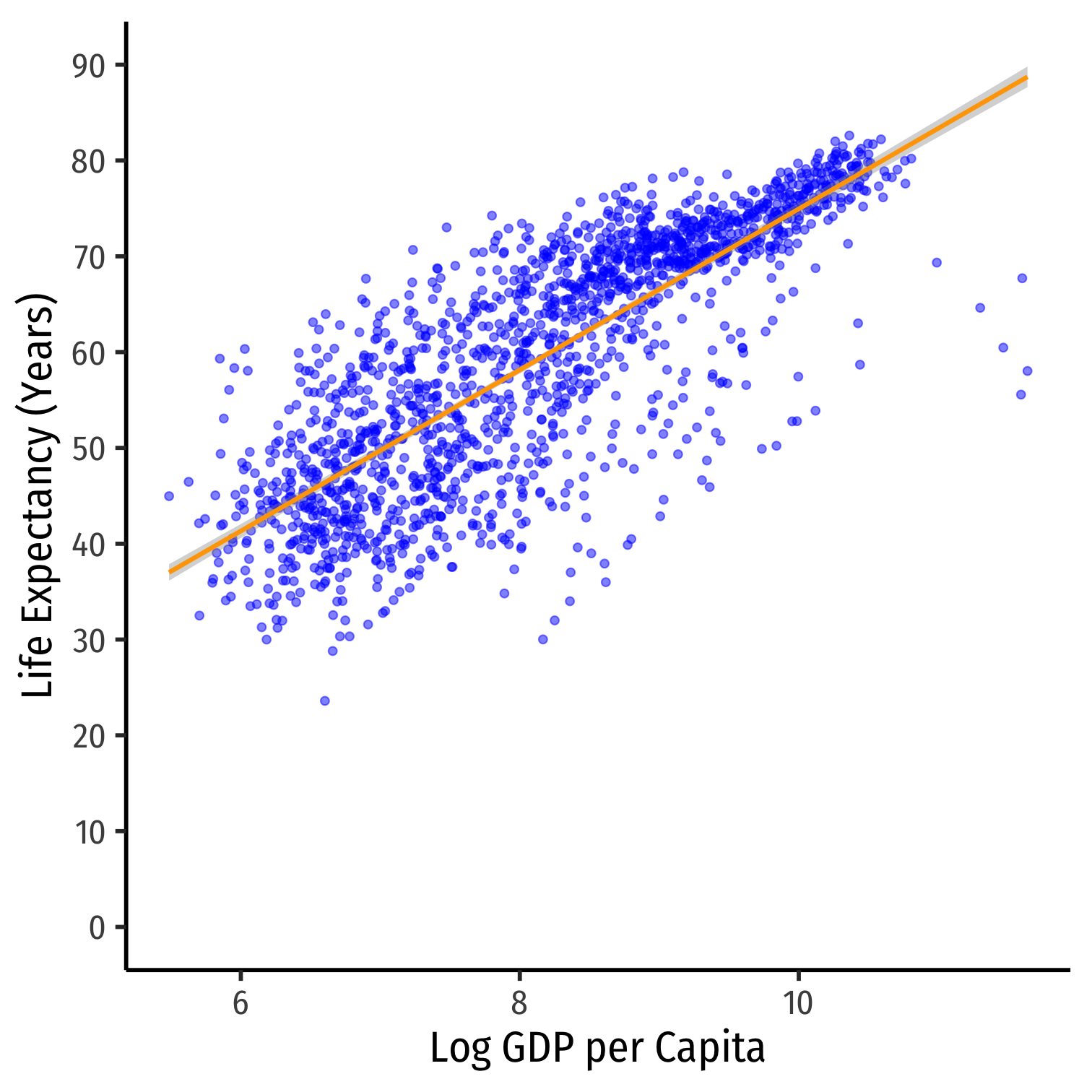 |
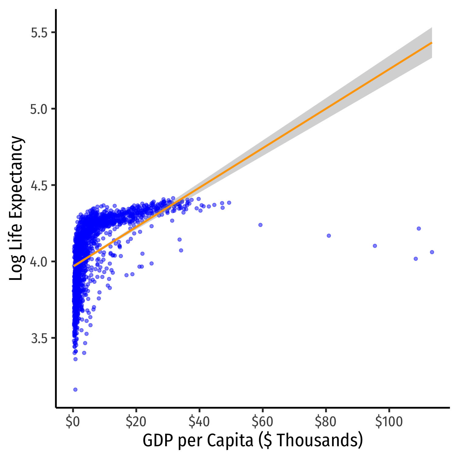 |
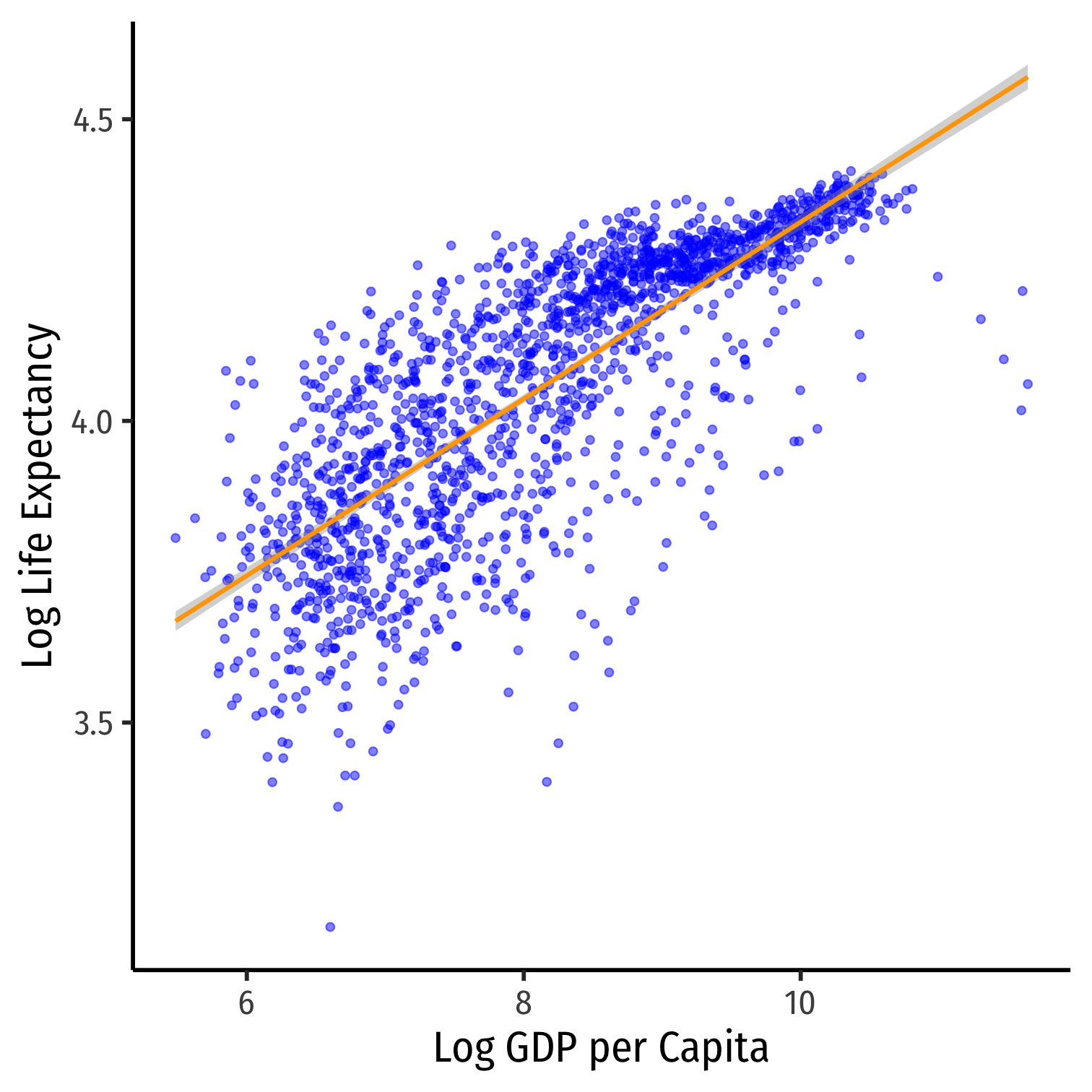 |
| ^Yi=^β0+^β1ln(Xi) | ln(^Yi)=^β0+^β1Xi | ln(^Yi)=^β0+^β1ln(Xi) |
| R2=0.65 | R2=0.30 | R2=0.61 |
We will do another set of R practice problems, and you will be given HW 5 to work on this material.
Slides
R Practice Problems
We will do some R Practice Problems on nonlinear models, which we will continue into Tuesday November 26.
Problem Set 4 Due TODAY
Problm Set 4 (on classes 3.1-3.5) is due TODAY.