3.9: Logarithmic Regression
ECON 480 · Econometrics · Fall 2019
Ryan Safner
Assistant Professor of Economics
safner@hood.edu
ryansafner/metricsf19
metricsF19.classes.ryansafner.com
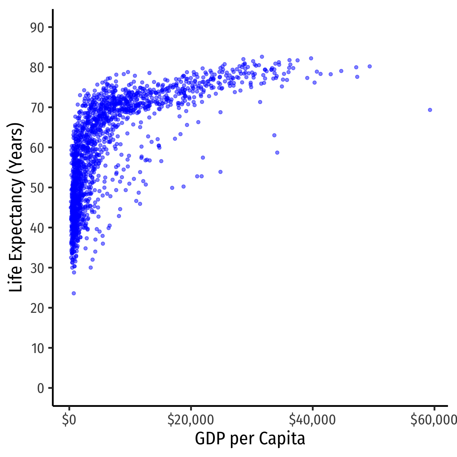
Nonlinearities
- Consider the
gapminderexample again
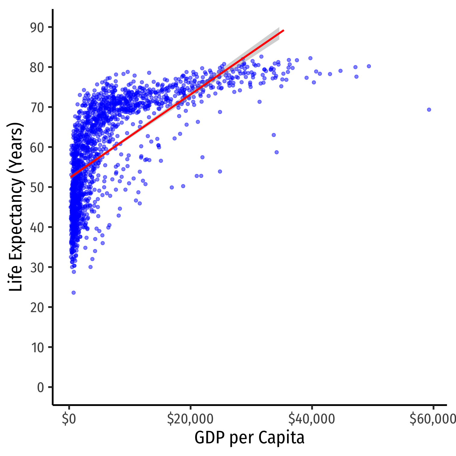
Nonlinearities
- Consider the
gapminderexample again- linear model
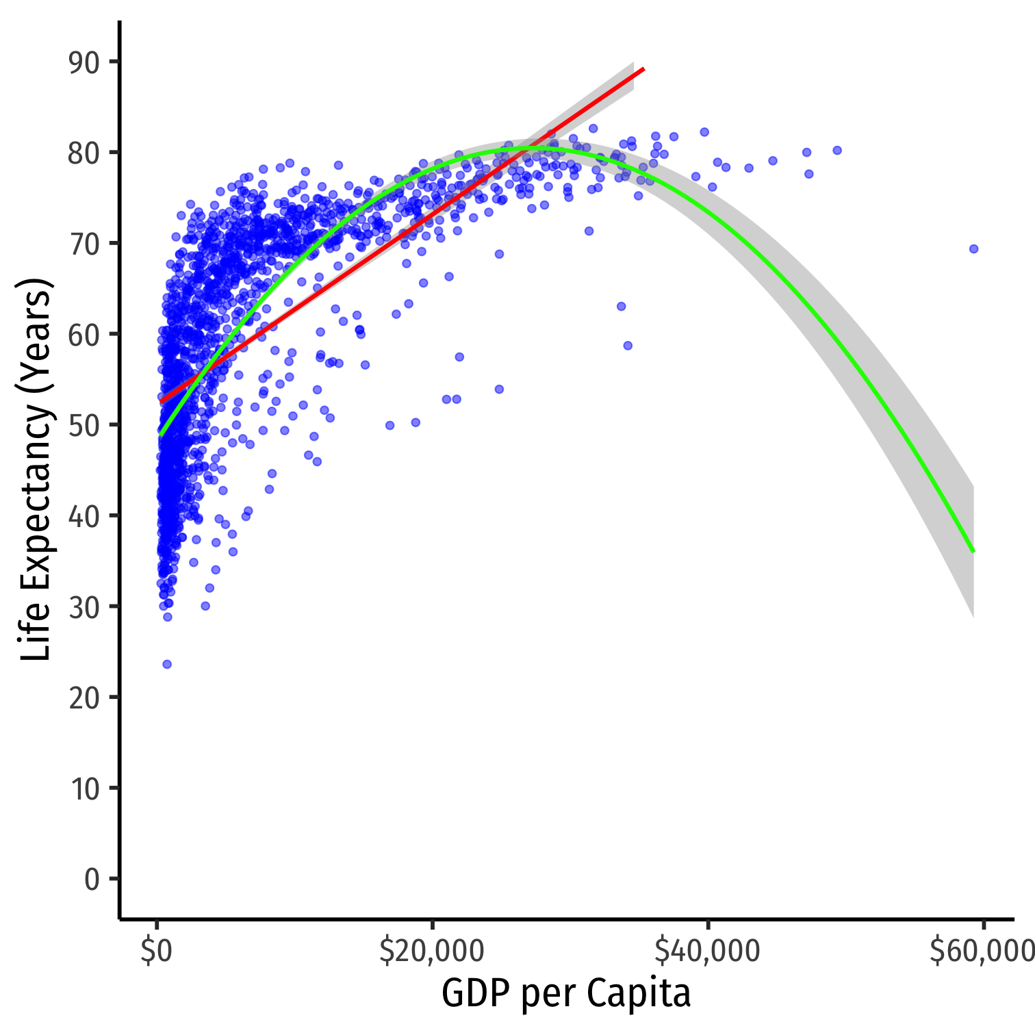
Nonlinearities
- Consider the
gapminderexample again- linear model
- polynomial model (quadratic)
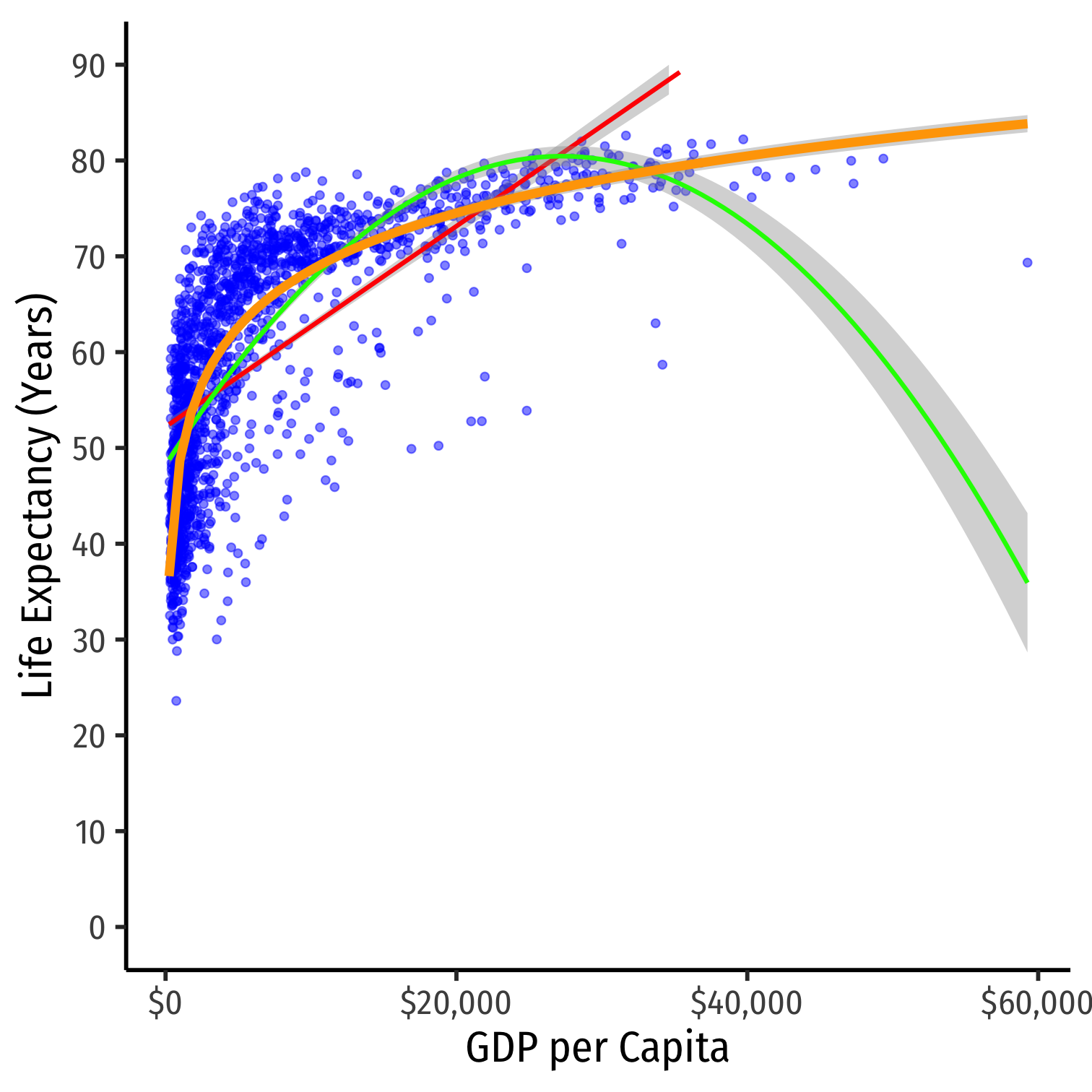
Nonlinearities
- Consider the
gapminderexample again- linear model
- polynomial model (quadratic)
- logarithmic model
Logarithmic Models
Logarithmic Models
Another model specification for nonlinear data is the logarithmic model1
- We transform either X, Y, or both by taking the (natural) logarithm
Logarithmic model has two additional advantages
- We can easily interpret coefficients as percentage changes or elasticities
- Useful economic shape: diminishing returns (production functions, utility functions, etc)
1 Note, this should not be confused with a logistic model, which is a model for dependent dummy variables.
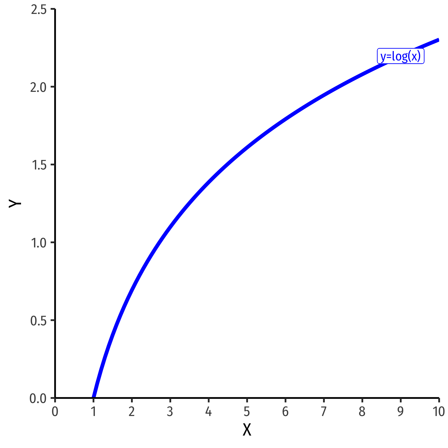
The Natural Logarithm
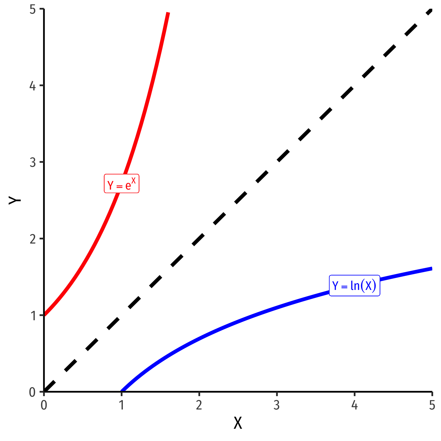
The exponential function, Y=eX or Y=exp(X), where base e=2.71828...
Natural logarithm is the inverse, Y=ln(X)
The Natural Logarithm: Review I
- Exponents are defined as
bn=b×b×⋯×b⏟n times
- where base b is multiplied by itself n times
The Natural Logarithm: Review I
- Exponents are defined as
bn=b×b×⋯×b⏟n times
- where base b is multiplied by itself n times
- Example: 23=2×2×2⏟n=3=8
The Natural Logarithm: Review I
- Exponents are defined as
bn=b×b×⋯×b⏟n times
- where base b is multiplied by itself n times
Example: 23=2×2×2⏟n=3=8
Logarithms are the inverse, defined as the exponents in the expressions above If bn=y, then logb(y)=n
- n is the number you must raise b to in order to get y
Example: log2(8)=3
The Natural Logarithm: Review II
- Logarithms can have any base, but common to use the natural logarithm (ln) with base e=2.71828...
If en=y, then ln(y)=n
The Natural Logarithm: Properties
- Natural logs have a lot of useful properties:
ln(1x)=−ln(x)
ln(ab)=ln(a)+ln(b)
ln(xa)=ln(x)−ln(a)
ln(xa)=aln(x)
dlnxdx=1x
The Natural Logarithm: Example
- Most useful property: for small change in x, Δx:
ln(x+Δx)−ln(x)⏟Difference in logs≈Δxx⏟Relative change
The Natural Logarithm: Example
- Most useful property: for small change in x, Δx:
ln(x+Δx)−ln(x)⏟Difference in logs≈Δxx⏟Relative change
Example: Let x=100 and Δx=1, relative change is:
Δxx=(101−100)100=0.01 or 1%
- The logged difference:
ln(101)−ln(100)=0.00995≈1%
The Natural Logarithm: Example
- Most useful property: for small change in x, Δx:
ln(x+Δx)−ln(x)⏟Difference in logs≈Δxx⏟Relative change
Example: Let x=100 and Δx=1, relative change is:
Δxx=(101−100)100=0.01 or 1%
- The logged difference:
ln(101)−ln(100)=0.00995≈1%
- This allows us to very easily interpret coefficients as percent changes or elasticities
Elasticity
An elasticity between two variables, EY,X describes the responsiveness of one variable to a change in another
Measured in percentages: a 1% change in X will cause a E% change in Y
Elasticity
An elasticity between two variables, EY,X describes the responsiveness of one variable to a change in another
Measured in percentages: a 1% change in X will cause a E% change in Y
EY,X=%ΔY%ΔX=(ΔYY)(ΔXX)
Elasticity
An elasticity between two variables, EY,X describes the responsiveness of one variable to a change in another
Measured in percentages: a 1% change in X will cause a E% change in Y
EY,X=%ΔY%ΔX=(ΔYY)(ΔXX)
- Numerator is relative change in Y, Denominator is relative change in X
Math FYI: Cobb Douglas Functions and Logs
- One of the (many) reasons why economists love Cobb-Douglas functions:
Y=ALαKβ
Math FYI: Cobb Douglas Functions and Logs
One of the (many) reasons why economists love Cobb-Douglas functions: Y=ALαKβ
Taking logs, relationship becomes linear:
Math FYI: Cobb Douglas Functions and Logs
One of the (many) reasons why economists love Cobb-Douglas functions: Y=ALαKβ
Taking logs, relationship becomes linear:
ln(Y)=ln(A)+αln(L)+βln(K)
Math FYI: Cobb Douglas Functions and Logs
One of the (many) reasons why economists love Cobb-Douglas functions: Y=ALαKβ
Taking logs, relationship becomes linear:
ln(Y)=ln(A)+αln(L)+βln(K)
- With data on (Y,L,K) and linear regression, can estimate α and β
- α: elasticity of Y with respect to L
- A 1% change in L will lead to an α% change in Y
- β: elasticity of Y with respect to K
- A 1% change in K will lead to a β% change in Y
- α: elasticity of Y with respect to L
Logarithms in R I
- The
log()function can easily take the logarithm
gapminder<-gapminder %>% mutate(loggdp=log(gdpPercap)) # log GDP per capitagapminder %>% head() # look at it| ABCDEFGHIJ0123456789 |
country <fctr> | continent <fctr> | year <int> | lifeExp <dbl> | pop <int> | gdpPercap <dbl> | loggdp <dbl> |
|---|---|---|---|---|---|---|
| Afghanistan | Asia | 1952 | 28.801 | 8425333 | 779.4453 | 6.658583 |
| Afghanistan | Asia | 1957 | 30.332 | 9240934 | 820.8530 | 6.710344 |
| Afghanistan | Asia | 1962 | 31.997 | 10267083 | 853.1007 | 6.748878 |
| Afghanistan | Asia | 1967 | 34.020 | 11537966 | 836.1971 | 6.728864 |
| Afghanistan | Asia | 1972 | 36.088 | 13079460 | 739.9811 | 6.606625 |
| Afghanistan | Asia | 1977 | 38.438 | 14880372 | 786.1134 | 6.667101 |
Logarithms in R II
- Note,
log()by default is the natural logarithm ln(), i.e. basee- Can change base with e.g.
log(x, base = 5) - Some common built-in logs:
log10,log2
- Can change base with e.g.
log10(100)## [1] 2log2(16)## [1] 4log(19683, base=3)## [1] 9Types of Logarithmic Models
- Three types of log regression models, depending on which variables we log
Types of Logarithmic Models
- Three types of log regression models, depending on which variables we log
- Linear-log model: Yi=β0+β1 ln(Xi)
Types of Logarithmic Models
- Three types of log regression models, depending on which variables we log
Linear-log model: Yi=β0+β1 ln(Xi)
Log-linear model: ln(Yi) =β0+β1Xi
Types of Logarithmic Models
- Three types of log regression models, depending on which variables we log
Linear-log model: Yi=β0+β1 ln(Xi)
Log-linear model: ln(Yi) =β0+β1Xi
Log-log model: ln(Yi) =β0+β1 ln(Xi)
Linear-Log Model
- Linear-log model has an independent variable (X) that is logged
Linear-Log Model
- Linear-log model has an independent variable (X) that is logged
Y=β0+β1ln(X)β1=ΔY(ΔXX)
Linear-Log Model
- Linear-log model has an independent variable (X) that is logged
Y=β0+β1ln(X)β1=ΔY(ΔXX)
- Marginal effect of X→Y: a 1% change in X→ a β1100 unit change in Y
Linear-Log Model in R
lin_log_reg<-lm(lifeExp~loggdp, data = gapminder)library(broom)tidy(lin_log_reg)| ABCDEFGHIJ0123456789 |
term <chr> | estimate <dbl> | std.error <dbl> | |
|---|---|---|---|
| (Intercept) | -9.100889 | 1.227674 | |
| loggdp | 8.405085 | 0.148762 |
^Life Expectancyi=−9.10+9.41ln(GDP)i
- A 1% change in GDP → a 9.41100= 0.0941 year increase in Life Expectancy
Linear-Log Model in R
lin_log_reg<-lm(lifeExp~loggdp, data = gapminder)library(broom)tidy(lin_log_reg)| ABCDEFGHIJ0123456789 |
term <chr> | estimate <dbl> | std.error <dbl> | |
|---|---|---|---|
| (Intercept) | -9.100889 | 1.227674 | |
| loggdp | 8.405085 | 0.148762 |
^Life Expectancyi=−9.10+9.41ln(GDP)i
A 1% change in GDP → a 9.41100= 0.0941 year increase in Life Expectancy
A 25% fall in GDP → a (−25×0.0941)= 2.353 year decrease in Life Expectancy
A 100% rise in GDP → a (100×0.0941)= 9.041 year increase in Life Expectancy
Linear-Log Model Graph I
ggplot(data = gapminder)+ aes(x = gdpPercap, y = lifeExp)+ geom_point(color="blue", alpha=0.5)+ geom_smooth(method="lm", formula=y~log(x), color="orange")+ scale_x_continuous(labels=scales::dollar, breaks=seq(0,120000,20000))+ scale_y_continuous(breaks=seq(0,90,10), limits=c(0,90))+ labs(x = "GDP per Capita", y = "Life Expectancy (Years)")+ theme_classic(base_family = "Fira Sans Condensed", base_size=20)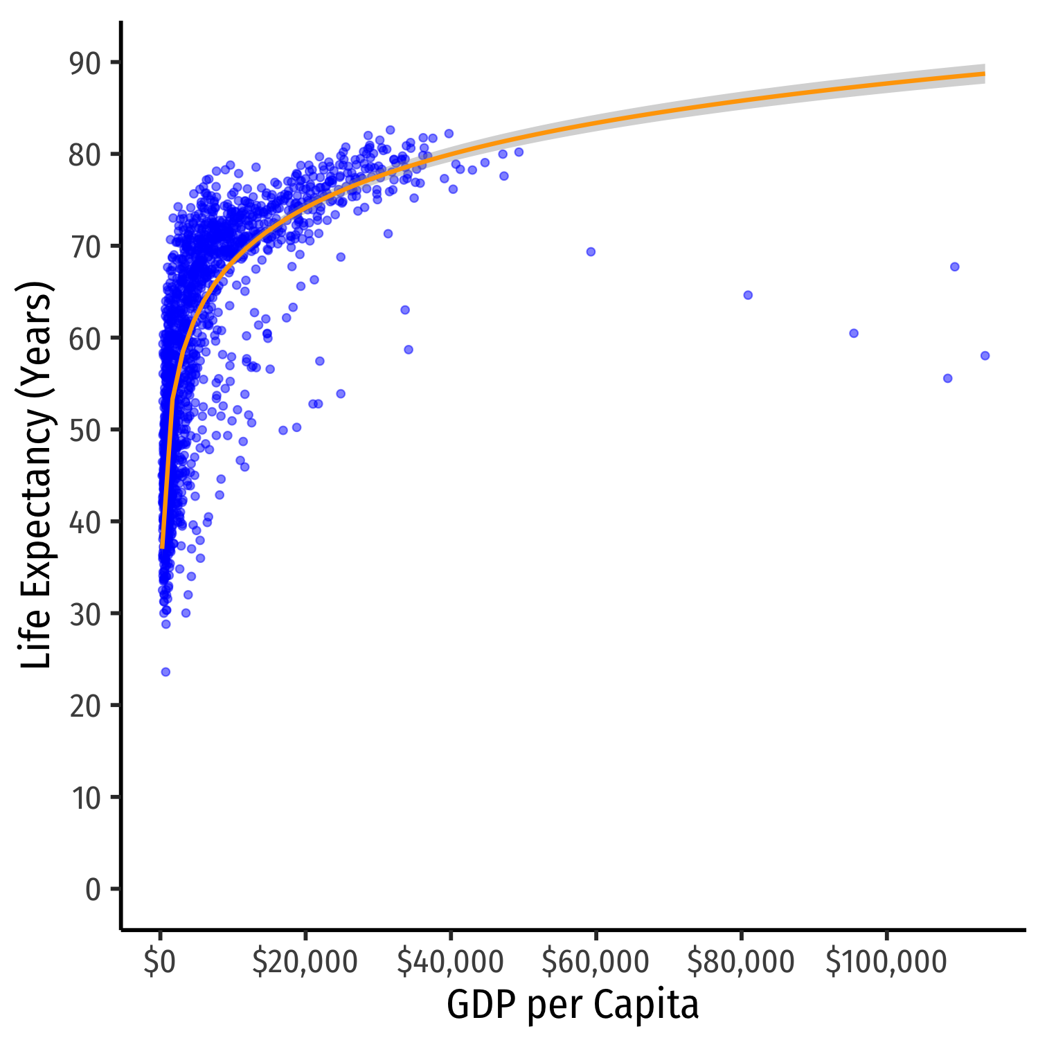
Linear-Log Model Graph II
ggplot(data = gapminder)+ aes(x = loggdp, y = lifeExp)+ geom_point(color="blue", alpha=0.5)+ geom_smooth(method="lm", color="orange")+ scale_y_continuous(breaks=seq(0,90,10), limits=c(0,90))+ labs(x = "Log GDP per Capita", y = "Life Expectancy (Years)")+ theme_classic(base_family = "Fira Sans Condensed", base_size=20)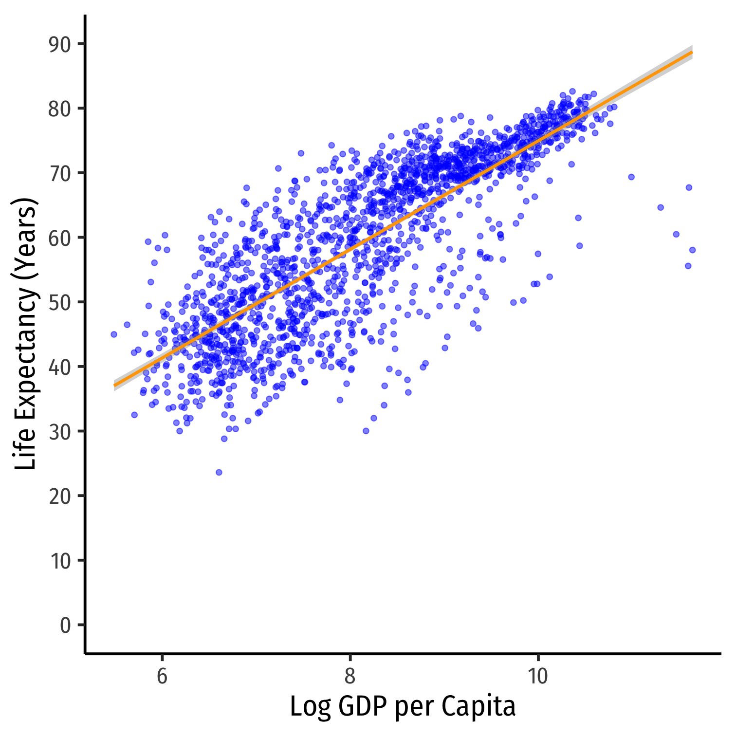
Log-Linear Model
- Log-linear model has the dependent variable (Y) logged
Log-Linear Model
- Log-linear model has the dependent variable (Y) logged
ln(Y)=β0+β1Xβ1=(ΔYY)ΔX
Log-Linear Model
- Log-linear model has the dependent variable (Y) logged
ln(Y)=β0+β1Xβ1=(ΔYY)ΔX
- Marginal effect of X→Y: a 1 unit change in X→ a β1×100 % change in Y
Log-Linear Model in R (Preliminaries)
We will again have very large/small coefficients if we deal with GDP directly, again let's transform
gdpPercapinto $1,000s, call itgdp_tThen log LifeExp
Log-Linear Model in R (Preliminaries)
We will again have very large/small coefficients if we deal with GDP directly, again let's transform
gdpPercapinto $1,000s, call itgdp_tThen log LifeExp
gapminder <- gapminder %>% mutate(gdp_t=gdpPercap/1000, # first make GDP/capita in $1000s loglife=log(lifeExp)) # take the log of LifeExpgapminder %>% head() # look at it| ABCDEFGHIJ0123456789 |
country <fctr> | continent <fctr> | year <int> | lifeExp <dbl> | pop <int> | gdpPercap <dbl> | loggdp <dbl> | gdp_t <dbl> | loglife <dbl> |
|---|---|---|---|---|---|---|---|---|
| Afghanistan | Asia | 1952 | 28.801 | 8425333 | 779.4453 | 6.658583 | 0.7794453 | 3.360410 |
| Afghanistan | Asia | 1957 | 30.332 | 9240934 | 820.8530 | 6.710344 | 0.8208530 | 3.412203 |
| Afghanistan | Asia | 1962 | 31.997 | 10267083 | 853.1007 | 6.748878 | 0.8531007 | 3.465642 |
| Afghanistan | Asia | 1967 | 34.020 | 11537966 | 836.1971 | 6.728864 | 0.8361971 | 3.526949 |
| Afghanistan | Asia | 1972 | 36.088 | 13079460 | 739.9811 | 6.606625 | 0.7399811 | 3.585960 |
| Afghanistan | Asia | 1977 | 38.438 | 14880372 | 786.1134 | 6.667101 | 0.7861134 | 3.649047 |
Log-Linear Model in R
log_lin_reg<-lm(loglife~gdp_t, data = gapminder)tidy(log_lin_reg)| ABCDEFGHIJ0123456789 |
term <chr> | estimate <dbl> | std.error <dbl> | |
|---|---|---|---|
| (Intercept) | 3.966639 | 0.0058345501 | |
| gdp_t | 0.012917 | 0.0004777072 |
^ln(Life Expectancy)i=3.967+0.013GDPi
Log-Linear Model in R
log_lin_reg<-lm(loglife~gdp_t, data = gapminder)tidy(log_lin_reg)| ABCDEFGHIJ0123456789 |
term <chr> | estimate <dbl> | std.error <dbl> | |
|---|---|---|---|
| (Intercept) | 3.966639 | 0.0058345501 | |
| gdp_t | 0.012917 | 0.0004777072 |
^ln(Life Expectancy)i=3.967+0.013GDPi
- A $1 (thousand) change in GDP → a 0.013×100%= 1.3% increase in Life Expectancy
Log-Linear Model in R
log_lin_reg<-lm(loglife~gdp_t, data = gapminder)tidy(log_lin_reg)| ABCDEFGHIJ0123456789 |
term <chr> | estimate <dbl> | std.error <dbl> | |
|---|---|---|---|
| (Intercept) | 3.966639 | 0.0058345501 | |
| gdp_t | 0.012917 | 0.0004777072 |
^ln(Life Expectancy)i=3.967+0.013GDPi
A $1 (thousand) change in GDP → a 0.013×100%= 1.3% increase in Life Expectancy
A $25 (thousand) fall in GDP → a (−25×1.3%)= 32.5% decrease in Life Expectancy
A $100 (thousand) rise in GDP → a (100×1.3%)= 130% increase in Life Expectancy
Linear-Log Model Graph I
ggplot(data = gapminder)+ aes(x = gdp_t, y = loglife)+ geom_point(color="blue", alpha=0.5)+ geom_smooth(method="lm", color="orange")+ scale_x_continuous(labels=scales::dollar, breaks=seq(0,120,20))+ labs(x = "GDP per Capita ($ Thousands)", y = "Log Life Expectancy")+ theme_classic(base_family = "Fira Sans Condensed", base_size=20)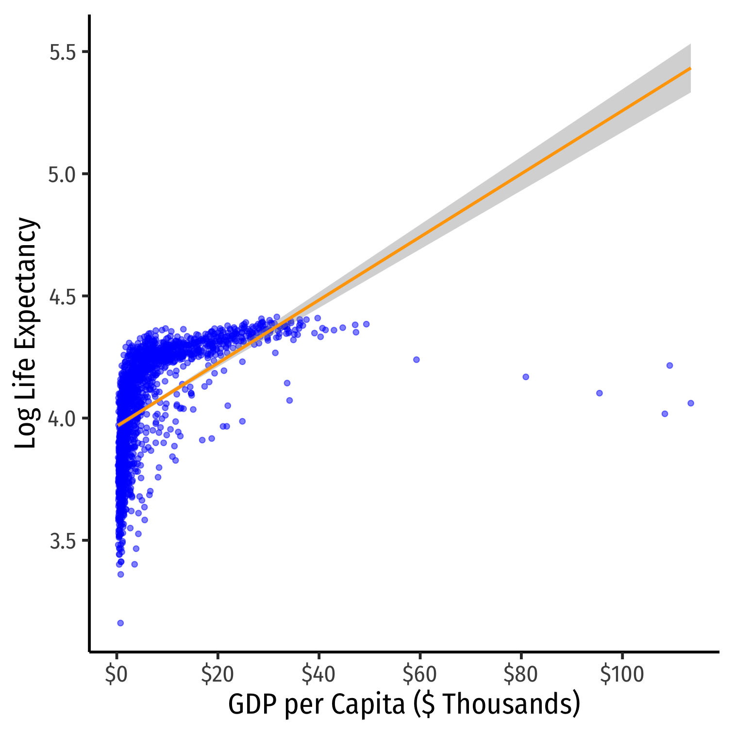
Log-Log Model
- Log-log model has both variables (X and Y) logged
Log-Log Model
- Log-log model has both variables (X and Y) logged
ln(Y)=β0+β1ln(X)β1=(ΔYY)(ΔXX)
Log-Log Model
- Log-log model has both variables (X and Y) logged
ln(Y)=β0+β1ln(X)β1=(ΔYY)(ΔXX)
Marginal effect of X→Y: a 1% change in X→ a β1 % change in Y
β1 is the elasticity of Y with respect to X!
Log-Log Model in R
log_log_reg<-lm(loglife~loggdp, data = gapminder)tidy(log_log_reg)| ABCDEFGHIJ0123456789 |
term <chr> | estimate <dbl> | std.error <dbl> | |
|---|---|---|---|
| (Intercept) | 2.864177 | 0.02328274 | |
| loggdp | 0.146549 | 0.00282126 |
^ln(Life Expectancy)i=2.864+0.147ln(GDP)i
Log-Log Model in R
log_log_reg<-lm(loglife~loggdp, data = gapminder)tidy(log_log_reg)| ABCDEFGHIJ0123456789 |
term <chr> | estimate <dbl> | std.error <dbl> | |
|---|---|---|---|
| (Intercept) | 2.864177 | 0.02328274 | |
| loggdp | 0.146549 | 0.00282126 |
^ln(Life Expectancy)i=2.864+0.147ln(GDP)i
- A 1% change in GDP → a 0.147% increase in Life Expectancy
Log-Log Model in R
log_log_reg<-lm(loglife~loggdp, data = gapminder)tidy(log_log_reg)| ABCDEFGHIJ0123456789 |
term <chr> | estimate <dbl> | std.error <dbl> | |
|---|---|---|---|
| (Intercept) | 2.864177 | 0.02328274 | |
| loggdp | 0.146549 | 0.00282126 |
^ln(Life Expectancy)i=2.864+0.147ln(GDP)i
A 1% change in GDP → a 0.147% increase in Life Expectancy
A 25% fall in GDP → a (−25×0.147%)= 3.675% decrease in Life Expectancy
A 100% rise in GDP → a (100×0.147%)= 14.7% increase in Life Expectancy
Log-Log Model Graph I
ggplot(data = gapminder)+ aes(x = loggdp, y = loglife)+ geom_point(color="blue", alpha=0.5)+ geom_smooth(method="lm", color="orange")+ labs(x = "Log GDP per Capita", y = "Log Life Expectancy")+ theme_classic(base_family = "Fira Sans Condensed", base_size=20)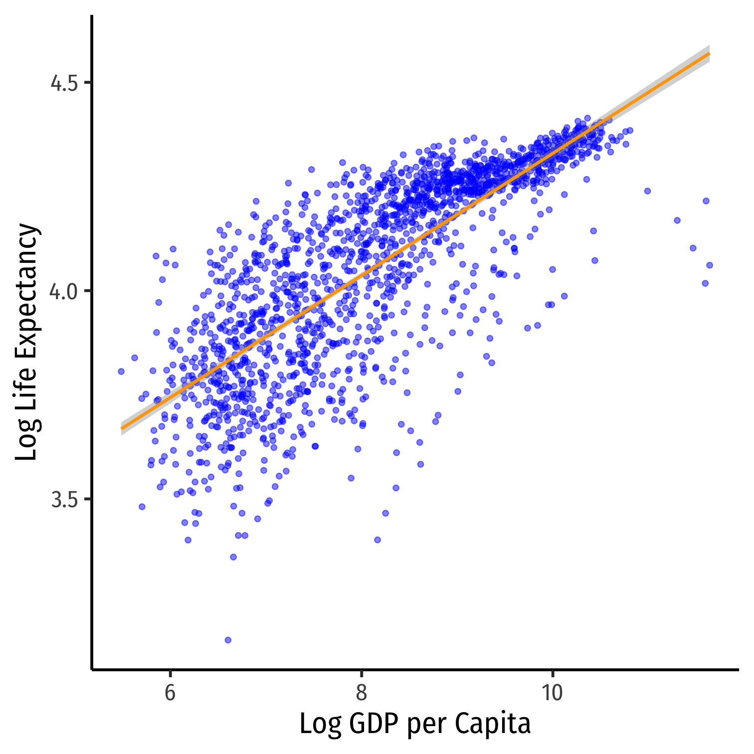
Comparing Models I
| Model | Equation | Interpretation |
|---|---|---|
| Linear-Log | Y=β0+β1ln(X) | 1% change in X→^β1100 unit change in Y |
| Log-Linear | ln(Y)=β0+β1X | 1 unit change in X→^β1×100% change in Y |
| Log-Log | ln(Y)=β0+β1ln(X) | 1% change in X→^β1% change in Y |
- Hint: the variable that gets logged changes in percent terms, the variable not logged changes in unit terms
Comparing Models II
library(huxtable)huxreg("Life Exp." = lin_log_reg, "Log Life Exp." = log_lin_reg, "Log Life Exp." = log_log_reg, coefs = c("Constant" = "(Intercept)", "GDP ($1000s)" = "gdp_t", "Log GDP" = "loggdp"), statistics = c("N" = "nobs", "R-Squared" = "r.squared", "SER" = "sigma"), number_format = 2)- Models are very different units, how to choose?
- Compare R2's
- Compare graphs
- Compare intution
| Life Exp. | Log Life Exp. | Log Life Exp. | |
| Constant | -9.10 *** | 3.97 *** | 2.86 *** |
| (1.23) | (0.01) | (0.02) | |
| GDP ($1000s) | 0.01 *** | ||
| (0.00) | |||
| Log GDP | 8.41 *** | 0.15 *** | |
| (0.15) | (0.00) | ||
| N | 1704 | 1704 | 1704 |
| R-Squared | 0.65 | 0.30 | 0.61 |
| SER | 7.62 | 0.19 | 0.14 |
| *** p < 0.001; ** p < 0.01; * p < 0.05. | |||
Comparing Models III
| Linear-Log | Log-Linear | Log-Log |
|---|---|---|
|
|
|
| ^Yi=^β0+^β1ln(Xi) | ln(^Yi)=^β0+^β1Xi | ln(^Yi)=^β0+^β1ln(Xi) |
| R2=0.65 | R2=0.30 | R2=0.61 |
When to Log?
- In practice, the following types of variables are logged:
- Variables that must always be positive (prices, sales, market values)
- Very large numbers (population, GDP)
- Variables we want to talk about as percentage changes or growth rates (money supply, population, GDP)
- Variables that have diminishing returns (output, utility)
- Variables that have nonlinear scatterplots
When to Log?
In practice, the following types of variables are logged:
- Variables that must always be positive (prices, sales, market values)
- Very large numbers (population, GDP)
- Variables we want to talk about as percentage changes or growth rates (money supply, population, GDP)
- Variables that have diminishing returns (output, utility)
- Variables that have nonlinear scatterplots
Avoid logs for:
- Variables that are less than one, decimals, 0, or negative
- Categorical variables (season, gender, political party)
- Time variables (year, week, day)
Comparing Across Units
Comparing Coefficients of Different Units I
^Yi=β0+β1X1+β2X2
We often want to compare coefficients to see which variable X1 or X2 has a bigger effect on Y
What if X1 and X2 are different units?
Example: ^Salaryi=β0+β1Batting averagei+β2Home runsi^Salaryi=−2,869,439.40+12,417,629.72Batting averagei+129,627.36Home runsi
Comparing Coefficients of Different Units II
- An easy way is to standardize the variables (i.e. take the Z-score)
Xstd=X−¯Xsd(X)
Comparing Coefficients of Different Units: Example
| Variable | Mean | Std. Dev. |
|---|---|---|
| Salary | $2,024,616 | $2,764,512 |
| Batting Average | 0.267 | 0.031 |
| Home Runs | 12.11 | 10.31 |
^Salaryi=−2,869,439.40+12,417,629.72Batting averagei+129,627.36Home runsi^Salaryistd=0.00+0.14Batting averagestdi+0.48Home runsstdi
- Marginal effect on Y (in standard deviations of Y) from 1 standard deviation change in X
- ^β1: a 1 standard deviation increase in Batting Average increases Salary by 0.14 standard deviations
- $0.14 \times 2,764,512=\$387,032$
- ^β2: a 1 standard deviation increase in Home Runs increases Salary by 0.48 standard deviations
- $0.48 \times 2,764,512=\$1,326,966$
Standardizing in R
- Use the
scale()command insidemutate()function to standardize a variable
gapminder<-gapminder %>% mutate(std_life = scale(lifeExp), std_gdp = scale(gdpPercap)) std_reg<-lm(std_life~std_gdp, data = gapminder)tidy(std_reg)| term | estimate | std.error | statistic | p.value |
| (Intercept) | 1.1e-16 | 0.0197 | 5.57e-15 | 1 |
| std_gdp | 0.584 | 0.0197 | 29.7 | 3.57e-156 |
Joint Hypothesis Testing
Joint Hypothesis Testing I
Example: Return again to:
^Wagei=^β0+^β1Male+^β2Northeasti+^β3Midwesti+^β4Southi
Joint Hypothesis Testing I
Example: Return again to:
^Wagei=^β0+^β1Male+^β2Northeasti+^β3Midwesti+^β4Southi
- Maybe region doesn't affect wages at all?
Joint Hypothesis Testing I
Example: Return again to:
^Wagei=^β0+^β1Male+^β2Northeasti+^β3Midwesti+^β4Southi
Maybe region doesn't affect wages at all?
H0:β2=0,β3=0,β4=0
Joint Hypothesis Testing I
Example: Return again to:
^Wagei=^β0+^β1Male+^β2Northeasti+^β3Midwesti+^β4Southi
Maybe region doesn't affect wages at all?
H0:β2=0,β3=0,β4=0
This is a joint hypothesis to test
Joint Hypothesis Testing II
- A joint hypothesis tests against the null hypothesis of a value for multiple parameters:
H0:β1=β2=0the hypotheses that multiple regressors are equal to zero (have no causal effect on the outcome)
Joint Hypothesis Testing II
A joint hypothesis tests against the null hypothesis of a value for multiple parameters: H0:β1=β2=0
the hypotheses that multiple regressors are equal to zero (have no causal effect on the outcome)Our alternative hypothesis is that: H1: either β1≠0 or β2≠0 or both
or simply, that H0 is not true
Types of Joint Hypothesis Tests
- Three main cases of joint hypothesis tests:
Types of Joint Hypothesis Tests
- Three main cases of joint hypothesis tests:
- H0: β1=β2=0
- Testing against the claim that multiple variables don't matter
- Useful under high multicollinearity between variables
- Ha: at least one parameter ≠ 0
Types of Joint Hypothesis Tests
- Three main cases of joint hypothesis tests:
H0: β1=β2=0
- Testing against the claim that multiple variables don't matter
- Useful under high multicollinearity between variables
- Ha: at least one parameter ≠ 0
H0: β1=β2
- Testing whether two variables matter the same
- Variables must be the same units
- Ha:β1(≠,<, or >)β2
H0: ALL β's =0
- The "Overall F-test"
- Testing against claim that regression model explains NO variation in Y
Joint Hypothesis Tests: F-statistic
- The F-statistic is the test-statistic used to test joint hypotheses about regression coefficients with an F-test
Joint Hypothesis Tests: F-statistic
The F-statistic is the test-statistic used to test joint hypotheses about regression coefficients with an F-test
This involves comparing two models:
- Unrestricted model: regression with all coefficients
- Restricted model: regression under null hypothesis (coefficients equal hypothesized values)
F is an analysis of variance (ANOVA)
- essentially tests whether R2 increases statistically significantly as we go from the restricted model$\rightarrow$unrestricted model
F has its own distribution, with two sets of degrees of freedom
Joint Hypothesis F-test: Example I
Example: Return again to:
^Wagei=^β0+^β1Malei+^β2Northeasti+^β3Midwesti+^β4Southi
Joint Hypothesis F-test: Example I
Example: Return again to:
^Wagei=^β0+^β1Malei+^β2Northeasti+^β3Midwesti+^β4Southi
- H0:β2=β3=β4=0
Joint Hypothesis F-test: Example I
Example: Return again to:
^Wagei=^β0+^β1Malei+^β2Northeasti+^β3Midwesti+^β4Southi
H0:β2=β3=β4=0
Ha: H0 is not true (at least one βi≠0)
Joint Hypothesis F-test: Example II
Example: Return again to:
^Wagei=^β0+^β1Malei+^β2Northeasti+^β3Midwesti+^β4Southi
- Unrestricted model:
^Wagei=^β0+^β1Malei+^β2Northeasti+^β3Midwesti+^β4Southi
Joint Hypothesis F-test: Example II
Example: Return again to:
^Wagei=^β0+^β1Malei+^β2Northeasti+^β3Midwesti+^β4Southi
- Unrestricted model:
^Wagei=^β0+^β1Malei+^β2Northeasti+^β3Midwesti+^β4Southi
- Restricted model:
^Wagei=^β0+^β1Malei
Joint Hypothesis F-test: Example II
Example: Return again to:
^Wagei=^β0+^β1Malei+^β2Northeasti+^β3Midwesti+^β4Southi
- Unrestricted model:
^Wagei=^β0+^β1Malei+^β2Northeasti+^β3Midwesti+^β4Southi
- Restricted model:
^Wagei=^β0+^β1Malei
- F: does going from restricted to unrestricted statistically significantly improve R2?
Calculating the F-statistic
Fq,(n−k−1)=((R2u−R2r)q)((1−R2u)(n−k−1))
Calculating the F-statistic
Fq,(n−k−1)=((R2u−R2r)q)((1−R2u)(n−k−1))
- R2u: the R2 from the unrestricted model (all variables)
Calculating the F-statistic
Fq,(n−k−1)=((R2u−R2r)q)((1−R2u)(n−k−1))
R2u: the R2 from the unrestricted model (all variables)
R2r: the R2 from the restricted model (null hypothesis)
Calculating the F-statistic
Fq,(n−k−1)=((R2u−R2r)q)((1−R2u)(n−k−1))
R2u: the R2 from the unrestricted model (all variables)
R2r: the R2 from the restricted model (null hypothesis)
q: number of restrictions (number of β′s=0 under null hypothesis)
Calculating the F-statistic
Fq,(n−k−1)=((R2u−R2r)q)((1−R2u)(n−k−1))
R2u: the R2 from the unrestricted model (all variables)
R2r: the R2 from the restricted model (null hypothesis)
q: number of restrictions (number of β′s=0 under null hypothesis)
k: number of X variables in unrestricted model (all variables)
F has two sets of degrees of freedom:
- q for the numerator
- (n−k−1) for the denominator
Calculating the F-statistic II
Fq,(n−k−1)=((R2u−R2r)q)((1−R2u)(n−k−1))
Key takeaway: The bigger the difference between (R2u−R2r), the greater the improvement in fit by adding variables, the larger the F!
This formula is (believe it or not) actually a simplified version (assuming homoskedasticity)
- I give you this formula to build your intuition of what F is measuring
F-test Example I
- We'll use the
wooldridgepackage'swage1data again
# load in data from wooldridge packagelibrary(wooldridge)wages<-wooldridge::wage1# run regressionsunrestricted_reg<-lm(wage~female+northcen+west+south, data=wages)restricted_reg<-lm(wage~female, data=wages)F-test Example II
- Unrestricted model:
^Wagei=^β0+^β1Femalei+^β2Northeasti+^β3Northcen+^β4Southi
- Restricted model:
^Wagei=^β0+^β1Femalei
H0:β2=β3=β4=0
q=3 restrictions (F numerator df)
n−k−1=526−4−1=521 (F denominator df)
F-test Example III
- We can use the
carpackage'slinearHypothesis()command to run an F-test:- first argument: name of the (unrestricted) regression
- second argument: vector of variable names (in quotes) you are testing
# load car package for additional regression toolslibrary("car") # F-testlinearHypothesis(unrestricted_reg, c("northcen", "west", "south"))| Res.Df | RSS | Df | Sum of Sq | F | Pr(>F) |
| 524 | 6.33e+03 | ||||
| 521 | 6.17e+03 | 3 | 157 | 4.43 | 0.00438 |
Second F-test Example: Are Two Coefficients Equal?
- The second type of test is whether two coefficients equal one another
Example:
^wagei=β0+β1Adolescent heighti+β2Adult heighti+β3Malei
Second F-test Example: Are Two Coefficients Equal?
- The second type of test is whether two coefficients equal one another
Example:
^wagei=β0+β1Adolescent heighti+β2Adult heighti+β3Malei
- Does height as an adolescent have the same effect on wages as height as an adult?
H0:β1=β2
Second F-test Example: Are Two Coefficients Equal?
- The second type of test is whether two coefficients equal one another
Example:
^wagei=β0+β1Adolescent heighti+β2Adult heighti+β3Malei
- Does height as an adolescent have the same effect on wages as height as an adult?
H0:β1=β2
- What is the restricted regression?
^wagei=β0+β1(Adolescent heighti+Adult heighti)+β3Malei
- q=1 restriction
Second F-test Example: Data
# load in dataheightwages<-read_csv("../data/heightwages.csv")# make a "heights" variable as the sum of adolescent (height81) and adult (height85) heightheightwages <- heightwages %>% mutate(heights=height81+height85)height_reg<-lm(wage96~height81+height85+male, data=heightwages)height_restricted_reg<-lm(wage96~heights+male, data=heightwages)Second F-test Example: Data
- For second argument, set two variables equal, in quotes
linearHypothesis(height_reg, "height81=height85") # F-test| Res.Df | RSS | Df | Sum of Sq | F | Pr(>F) |
| 6.59e+03 | 5.13e+06 | ||||
| 6.59e+03 | 5.13e+06 | 1 | 959 | 1.23 | 0.267 |
Insufficient evidence to reject H0!
The effect of adolescent and adult height on wages is the same
All F-test I
summary(unrestricted_reg)## ## Call:## lm(formula = wage ~ female + northcen + west + south, data = wages)## ## Residuals:## Min 1Q Median 3Q Max ## -6.3269 -2.0105 -0.7871 1.1898 17.4146 ## ## Coefficients:## Estimate Std. Error t value Pr(>|t|) ## (Intercept) 7.5654 0.3466 21.827 <2e-16 ***## female -2.5652 0.3011 -8.520 <2e-16 ***## northcen -0.5918 0.4362 -1.357 0.1755 ## west 0.4315 0.4838 0.892 0.3729 ## south -1.0262 0.4048 -2.535 0.0115 * ## ---## Signif. codes: 0 '***' 0.001 '**' 0.01 '*' 0.05 '.' 0.1 ' ' 1## ## Residual standard error: 3.443 on 521 degrees of freedom## Multiple R-squared: 0.1376, Adjusted R-squared: 0.131 ## F-statistic: 20.79 on 4 and 521 DF, p-value: 6.501e-16- Last line of regression output from
summary()of anlm()object is an All F-test- H0: all β′s=0
- the regression explains no variation in Y
- Calculates an
F-statisticthat, if high enough, is significant (p-value<0.05) enough to reject H0
All F-test II
- Alternatively, if you use
broominstead ofsummary()oflmobject:glance()command makes table of regression summary statisticstidy()only shows coefficients
library(broom)glance(unrestricted_reg)| r.squared | adj.r.squared | sigma | statistic | p.value | df | logLik | AIC | BIC | deviance | df.residual |
| 0.138 | 0.131 | 3.44 | 20.8 | 6.5e-16 | 5 | -1.39e+03 | 2.8e+03 | 2.83e+03 | 6.17e+03 | 521 |
- "statistic" is the All F-test, "p.value" next to it is the p value from the F test