3.6: Regression with Categorical Data - Class Notes
Contents
Tuesday, November 12, 2019
Overview
Today we look at how to use data that is categorical (i.e. variables that indicate an observation’s membership in a particular group or category). We introduce them into regression models as dummy variables that can equal 0 or 1: where 1 indicates membership in a category, and 0 indicates non-membership.
We also look at what happens when categorical variables have more than two values: for regression, we introduce a dummy variable for each possible category - but be sure to leave out one reference category to avoid the dummy variable trap.
Slides
Problem Set 4 Due Tuesday Nov 19
Problm Set 4 (on classes 3.1-3.5) is due by Thursday November 21.
Appendix: T-Test for Difference in Group Means
Often we want to compare the means between two groups, and see if the difference is statistically significant. As an example, is there a statistically significant difference in average hourly earnings between men and women? Let:
- μW: mean hourly earnings for female college graduates
- μM: mean hourly earnings for male college graduates
We want to run a hypothesis test for the difference (d) in these two population means:
μM−μW=d0
Our null hypothesis is that there is no statistically significant difference. Let’s also have a two-sided alternative hypothesis, simply that there is a difference (positive or negative).
- H0:d=0
- H1:d≠0
Note a logical one-sided alternative would be H2:d>0, i.e. men earn more than women
The Sampling Distribution of d
The true population means μM,μW are unknown, we must estimate them from samples of men and women. Let:
- ˉYM the average earnings of a sample of nM men
- ˉYW the average earnings of a sample of nW women
We then estimate (μM−μW) with the sample (ˉYM−ˉYW).
We would then run a t-test and calculate the test-statistic for the difference in means. The formula for the test statistic is:
t=(¯YM−¯YW)−d0√s2MnM+s2WnW
We then compare t against the critical value t∗, or calculate the p-value P(T>t) as usual to determine if we have sufficient evidence to reject H0
## ── Attaching packages ─────────────────────────────── tidyverse 1.2.1 ──## ✔ ggplot2 3.2.0 ✔ purrr 0.3.3
## ✔ tibble 2.1.3 ✔ dplyr 0.8.3
## ✔ tidyr 1.0.0 ✔ stringr 1.4.0
## ✔ readr 1.3.1 ✔ forcats 0.4.0## ── Conflicts ────────────────────────────────── tidyverse_conflicts() ──
## ✖ dplyr::filter() masks stats::filter()
## ✖ dplyr::lag() masks stats::lag()library(wooldridge)
# Our data comes from wage1 in the wooldridge package
wages<-wooldridge::wage1
# look at average wage for men
wages %>%
filter(female==0) %>%
summarize(average = mean(wage),
sd = sd(wage))## average sd
## 1 7.099489 4.160858# look at average wage for women
wages %>%
filter(female==1) %>%
summarize(average = mean(wage),
sd = sd(wage))## average sd
## 1 4.587659 2.529363So our data is telling us that male and female average hourly earnings are distributed as such:
ˉYM∼N(7.10,4.16)ˉYW∼N(4.59,2.53)
We can plot this to see visually. There is a lot of overlap in the two distributions, but the male average is higher than the female average, and there is also a lot more variation in males than females, noticeably the male distribution skews further to the right.
wages$female<-as.factor(wages$female)

library("ggplot2")
ggplot(data=wages,aes(x=wage,fill=female))+
  geom_density(alpha=0.5)+
  scale_x_continuous(seq(0,25,5),name="Wage",labels=scales::dollar)+
  theme_light()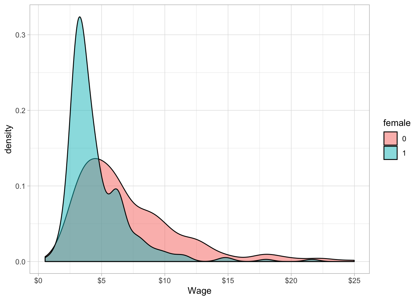
Knowing the distributions of male and female average hourly earnings, we can estimate the sampling distribution of the difference in group eans between men and women as:
The mean:
ˉd=ˉYM−ˉYWˉd=7.10−4.59ˉd=2.51
The standard error of the mean:
SE(ˉd)=√s2MnM+s2WnW=√4.162274+2.332252≈0.29
So the sampling distribution of the difference in group means is distributed:
ˉd∼N(2.51,0.29)
ggplot(data.frame(x=0:6),aes(x=x))+
  stat_function(fun=dnorm, args=list(mean=2.51, sd=0.29), color="purple")+
  ylab("Density")+
  scale_x_continuous(seq(0,6,1),name="Wage Difference",labels=scales::dollar)+
  theme_light()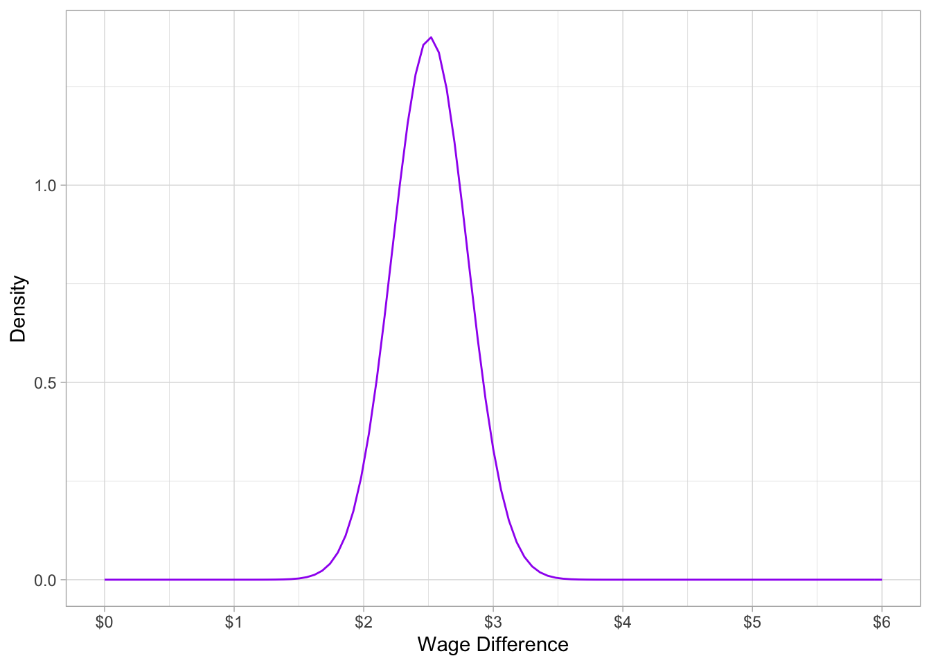
Now we the t-test like any other:
t=estimate−null hypothesisstandard error of the estimate=d−0SE(d)=2.51−00.29=8.66
This is statistically significant. The p-value, P(t>8.66)= is 0.000000000000000000410, or basically, 0.
## [1] 4.102729e-17The t-test in R
##
##  Welch Two Sample t-test
##
## data:  wage by female
## t = 8.44, df = 456.33, p-value = 4.243e-16
## alternative hypothesis: true difference in means is not equal to 0
## 95 percent confidence interval:
##  1.926971 3.096690
## sample estimates:
## mean in group 0 mean in group 1
## 7.099489 4.587659##
## Call:
## lm(formula = wage ~ female, data = wages)
##
## Residuals:
## Min 1Q Median 3Q Max
## -5.5995 -1.8495 -0.9877 1.4260 17.8805
##
## Coefficients:
## Estimate Std. Error t value Pr(>|t|)
## (Intercept) 7.0995 0.2100 33.806 < 2e-16 ***
## female1 -2.5118 0.3034 -8.279 1.04e-15 ***
## ---
## Signif. codes: 0 '***' 0.001 '**' 0.01 '*' 0.05 '.' 0.1 ' ' 1
##
## Residual standard error: 3.476 on 524 degrees of freedom
## Multiple R-squared: 0.1157, Adjusted R-squared: 0.114
## F-statistic: 68.54 on 1 and 524 DF, p-value: 1.042e-15