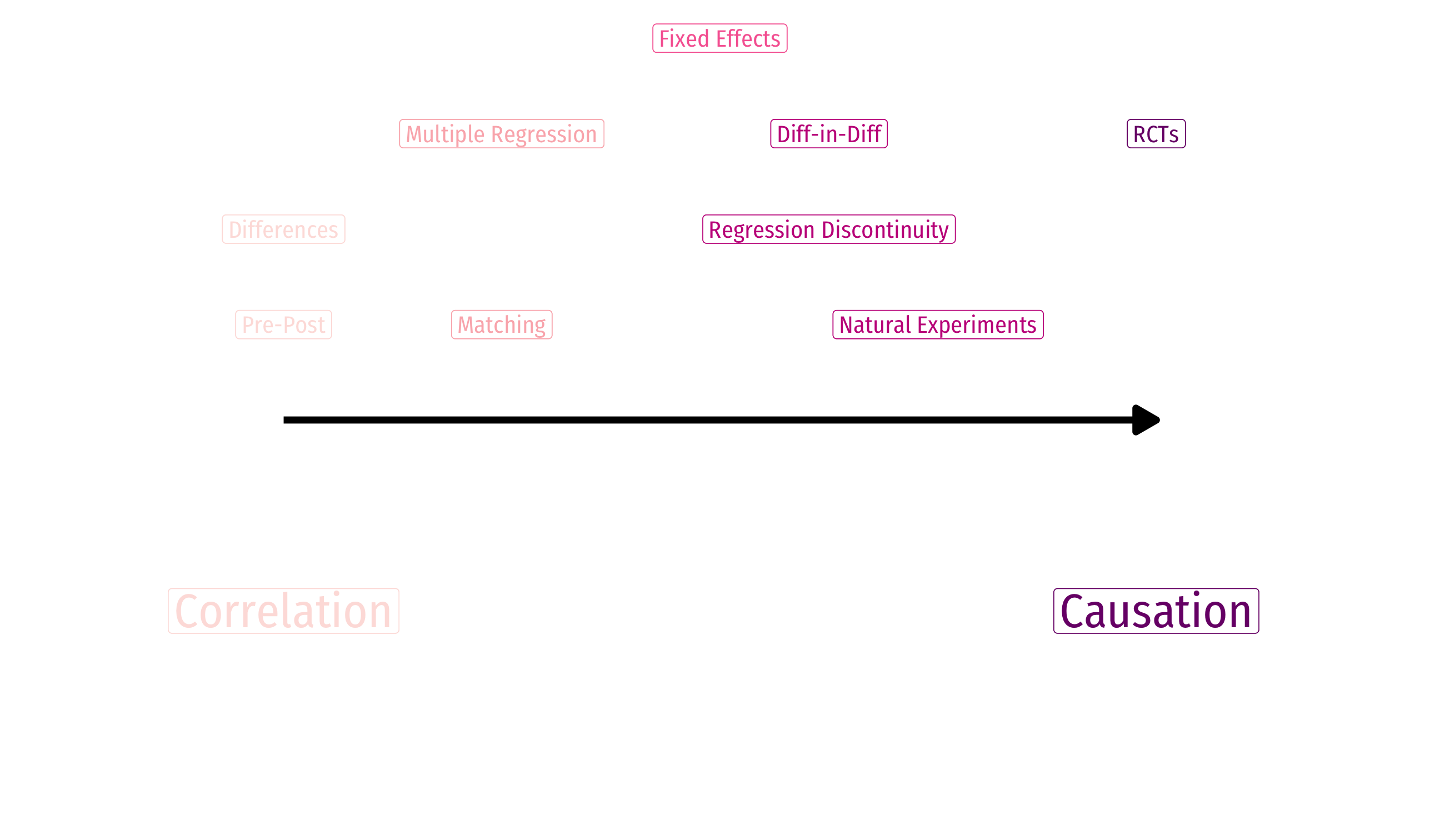
Clever Research Designs Identify Causality
Again, this toolkit of research designs to identify causal effects is the economist's comparative advantage that firms and governments want!
Difference-in-Difference Models I
Often, we want to examine the consequences of a change, such as a law or policy
Example: how do States that implement law X see changes in Y
- Treatment: States that implement law X
- Control: States that did not implement law X
If we have panel data with observations for all states before and after the change...
Find the difference between treatment & control groups in their differences before and after the treatment period

Visualizing Diff-in-Diff
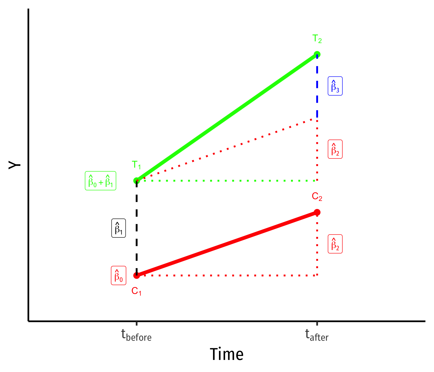
^Yit=β0+β1Treatedi+β2Aftert+β3(Treatedi×Aftert)+uit
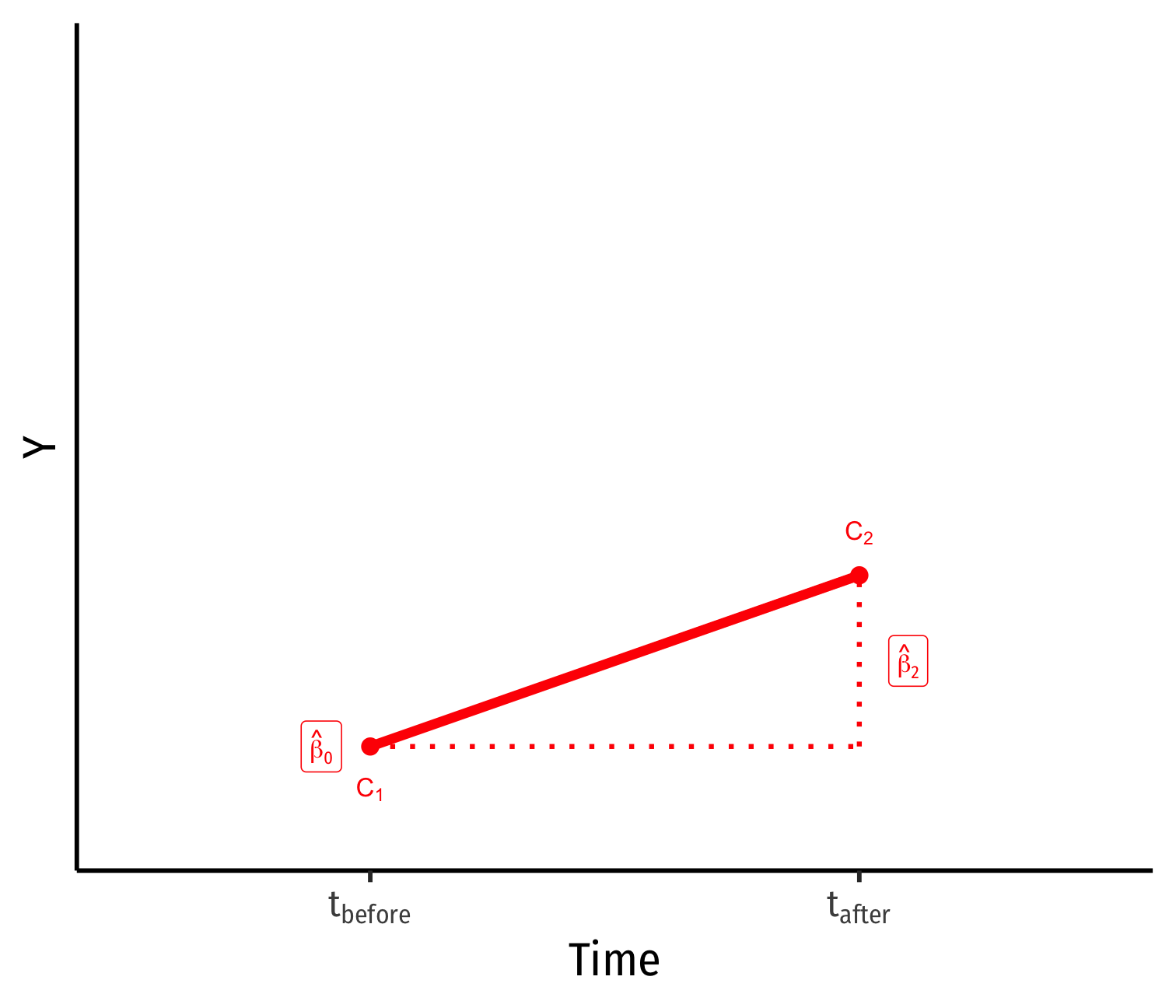
- Control group (Treated=0)
^β0: value of Y for control group before treatment
^β2: time difference (for control group)
Visualizing Diff-in-Diff
^Yit=β0+β1Treatedi+β2Aftert+β3(Treatedi×Aftert)+uit
- Control group (Treated=0)
^β0: value of Y for control group before treatment
^β2: time difference (for control group)
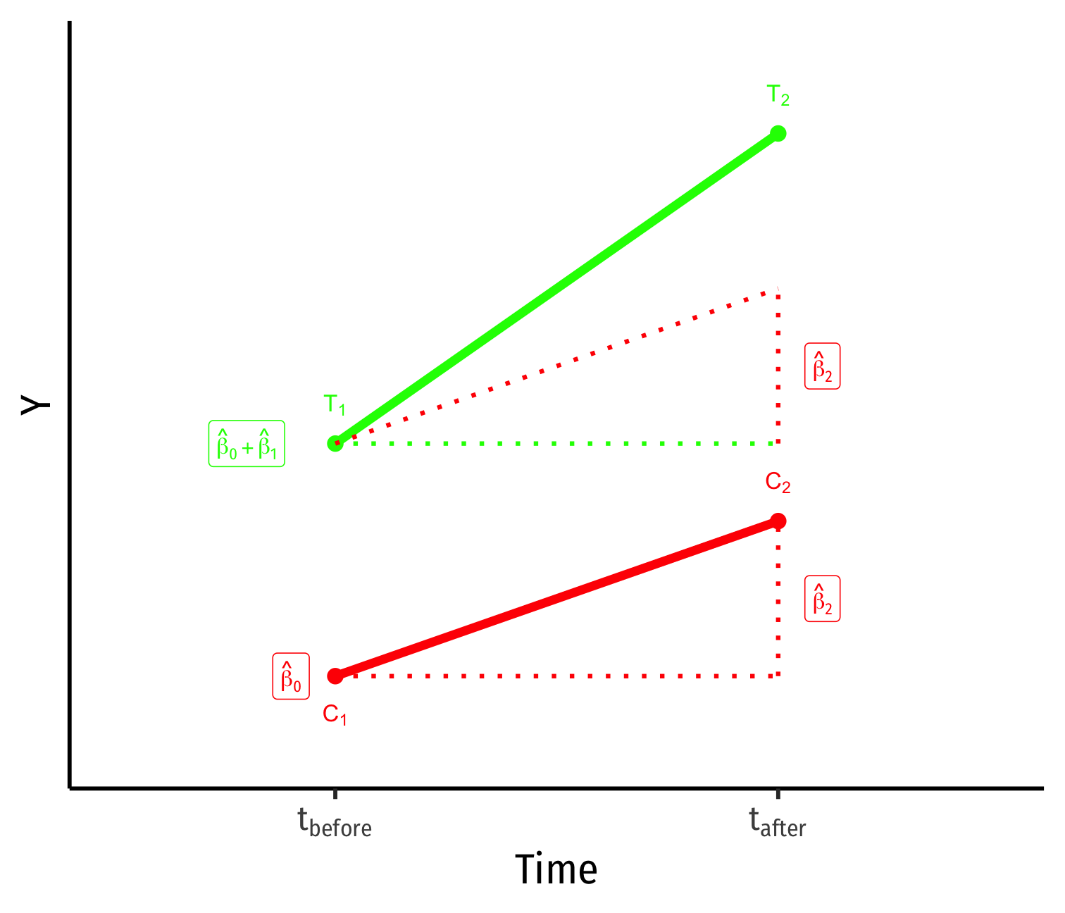
Treated group (Treated=1)
Visualizing Diff-in-Diff
^Yit=β0+β1Treatedi+β2Aftert+β3(Treatedi×Aftert)+uit
- Control group (Treated=0)
^β0: value of Y for control group before treatment
^β2: time difference (for control group)
Treated group (Treated=1)
^β1: difference between groups before treatment
Visualizing Diff-in-Diff
^Yit=β0+β1Treatedi+β2Aftert+β3(Treatedi×Aftert)+uit
- Control group (Treated=0)
^β0: value of Y for control group before treatment
^β2: time difference (for control group)
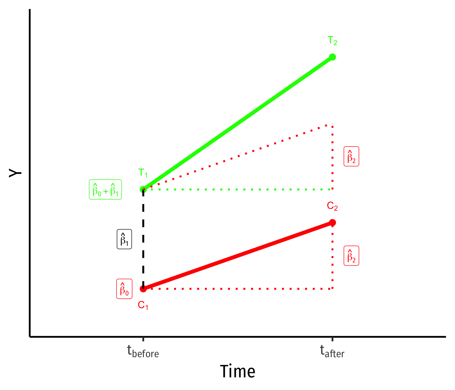
Treated group (Treated=1)
^β1: difference between groups before treatment
^β3: difference-in-difference: treatment effect
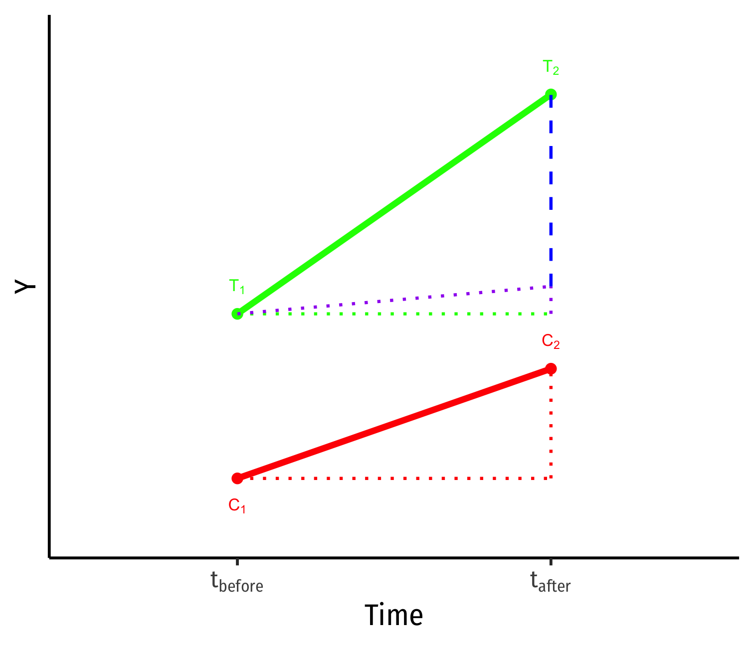
Visualizing Diff-in-Diff II
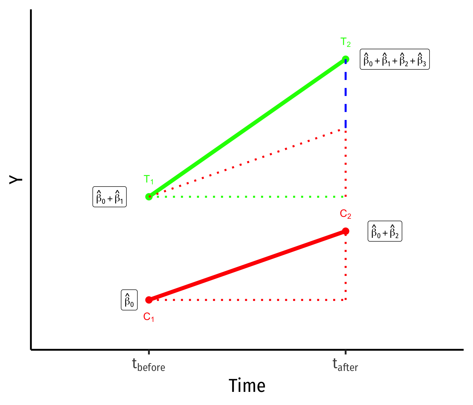
^Yit=β0+β1Treatedi+β2Aftert+β3(Treatedi×Aftert)+uit
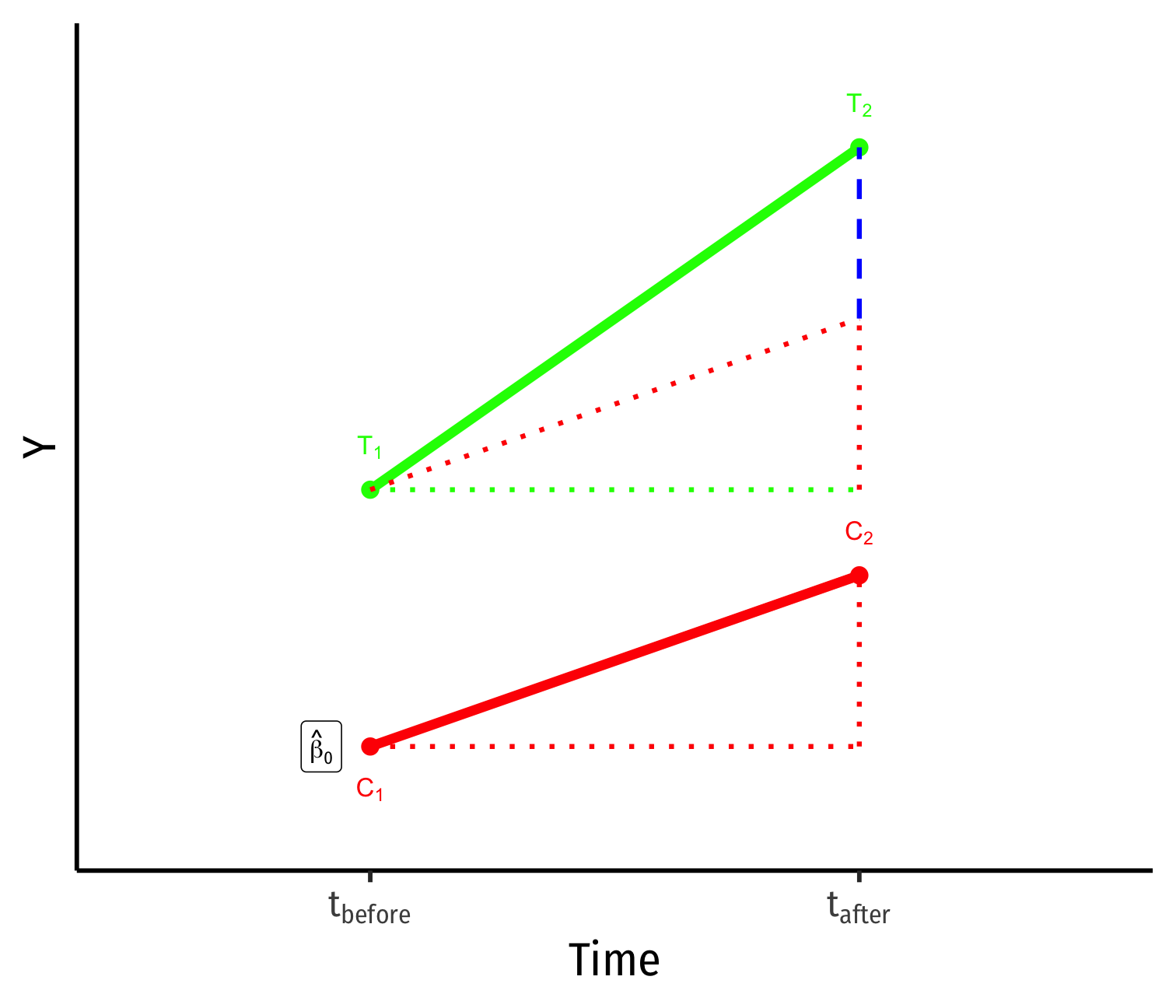
- Yi for Control group before: ^β0
Visualizing Diff-in-Diff II
^Yit=β0+β1Treatedi+β2Aftert+β3(Treatedi×Aftert)+uit
Yi for Control group before: ^β0
Yi for Control group after: ^β0+^β2
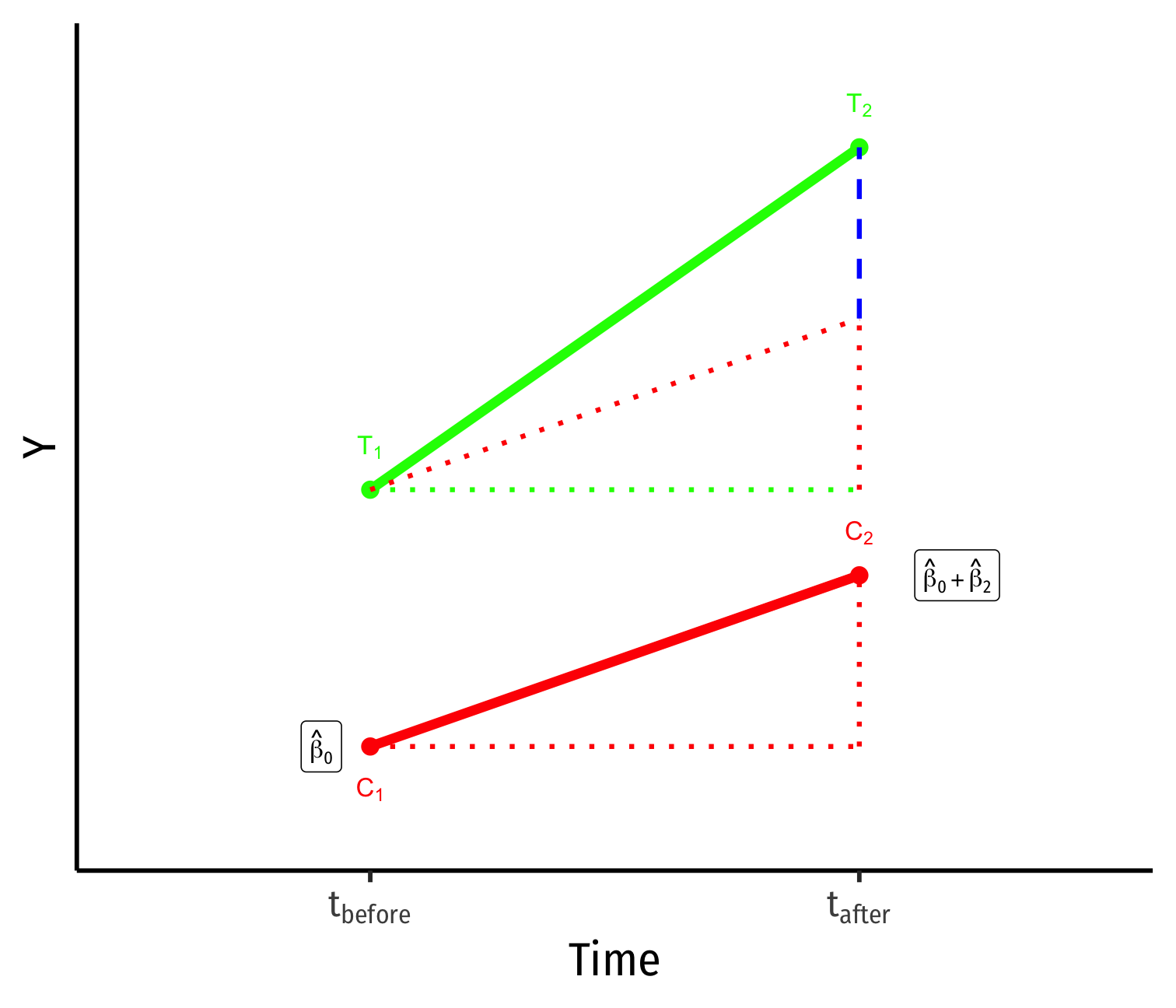
Visualizing Diff-in-Diff II
^Yit=β0+β1Treatedi+β2Aftert+β3(Treatedi×Aftert)+uit
Yi for Control group before: ^β0
Yi for Control group after: ^β0+^β2
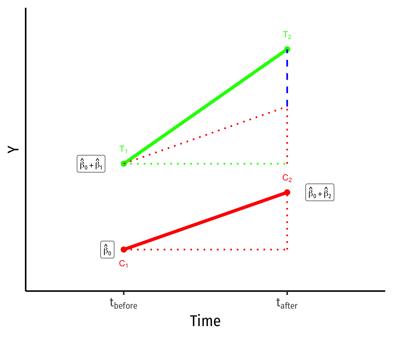
Yi for Treatment group before: ^β0+^β1
Visualizing Diff-in-Diff II
^Yit=β0+β1Treatedi+β2Aftert+β3(Treatedi×Aftert)+uit
Yi for Control group before: ^β0
Yi for Control group after: ^β0+^β2
Yi for Treatment group before: ^β0+^β1
Yi for Treatment group after: ^β0+^β1+^β2+^β3
Visualizing Diff-in-Diff II
^Yit=β0+β1Treatedi+β2Aftert+β3(Treatedi×Aftert)+uit
Yi for Control group before: ^β0
Yi for Control group after: ^β0+^β2
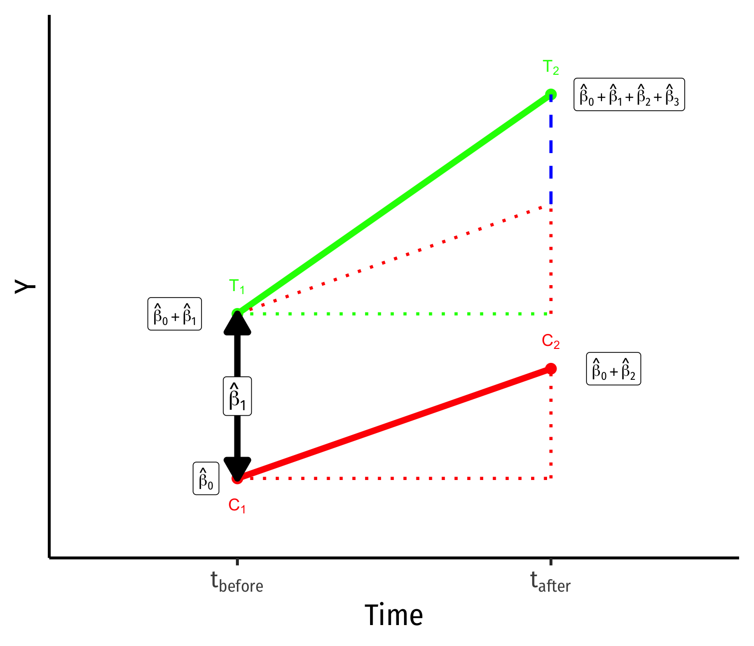
Yi for Treatment group before: ^β0+^β1
Yi for Treatment group after: ^β0+^β1+^β2+^β3
Group Difference (before): ^β1
Visualizing Diff-in-Diff II
^Yit=β0+β1Treatedi+β2Aftert+β3(Treatedi×Aftert)+uit
Yi for Control group before: ^β0
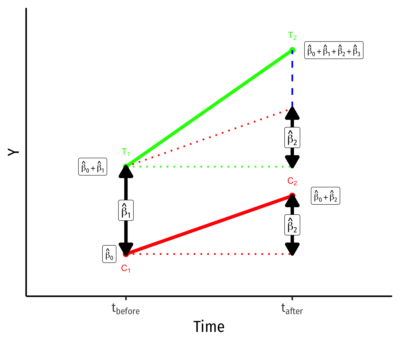
Yi for Control group after: ^β0+^β2
Yi for Treatment group before: ^β0+^β1
Yi for Treatment group after: ^β0+^β1+^β2+^β3
Group Difference (before): ^β1
Time Difference: ^β2
Visualizing Diff-in-Diff II
^Yit=β0+β1Treatedi+β2Aftert+β3(Treatedi×Aftert)+uit

Yi for Control group before: ^β0
Yi for Control group after: ^β0+^β2
Yi for Treatment group before: ^β0+^β1
Yi for Treatment group after: ^β0+^β1+^β2+^β3
Group Difference (before): ^β1
Time Difference: ^β2
Difference-in-difference: ^β3 (treatment effect)
Key Assumption: Counterfactual
^Yit=β0+β1Treatedi+β2Aftert+β3(Treatedi×Aftert)+uit
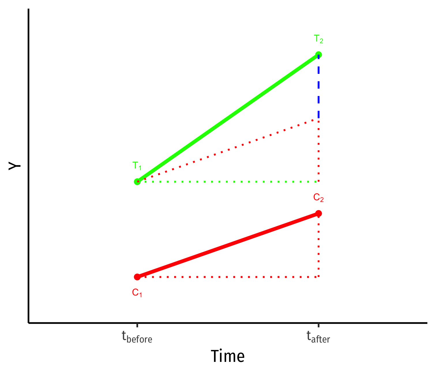
Key assumption for DND: time trends (for treatment and control) are parallel
Treatment and control groups assumed to be identical over time on average, except for treatment
Counterfactual: if the treatment group had not recieved treatment, it would have changed identically over time as the control group (^β2)
Key Assumption: Counterfactual
^Yit=β0+β1Treatedi+β2Aftert+β3(Treatedi×Aftert)+uit
- If the time-trends would have been different, a biased measure of the treatment effect (^β3)!
Example: Diff-in-Diff Graph
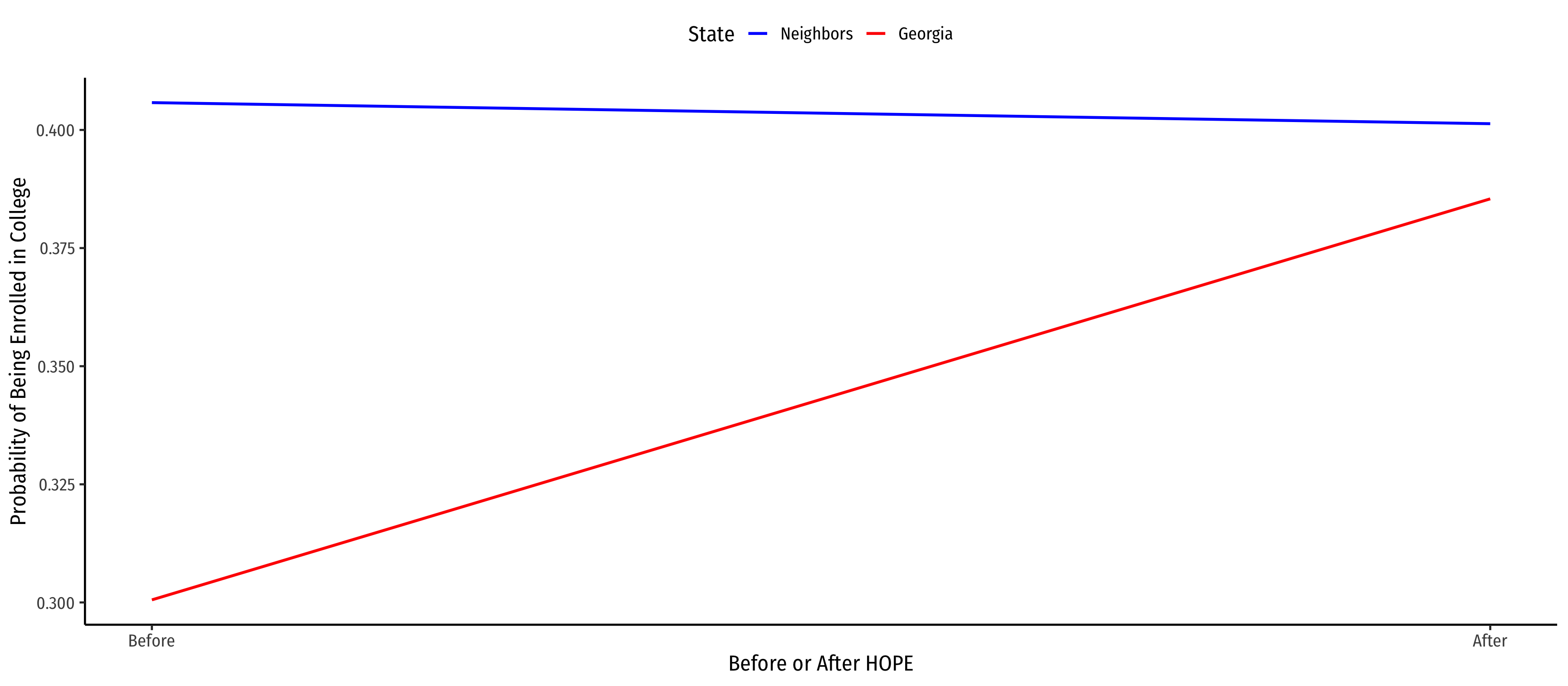
Card & Kreuger (1994): Background I
Card & Kreuger (1994) compare employment in fast food restaurants on New Jersey and Pennsylvania sides of border between February and November 1992.
Pennsylvania & New Jersey both had a minimum wage of $4.25 before February 1992
In February 1992, New Jersey raised minimum wage from $4.25 to $5.05

Card & Kreuger (1994): Background II
If we look only at New Jersey before & after change:
- Omitted variable bias: macroeconomic variables (there's a recession!), weather, etc.
- Including PA as a control will control for these time-varying effects if they are national trends
Surveyed 400 fast food restaurants on each side of the border, before & after min wage increase
- Key assumption: Pennsylvania and New Jersey follow parallel trends,
- Counterfactual: if not for the minimum wage increase, NJ employment would have changed similar to PA employment
Card & Kreuger (1994): Comparisons

Card & Kreuger (1994): Summary I

Card & Kreuger (1994): Summary II

Card & Kreuger (1994): Results
