3.7: Regression with Interaction Effects
ECON 480 · Econometrics · Fall 2019
Ryan Safner
Assistant Professor of Economics
safner@hood.edu
ryansafner/metricsf19
metricsF19.classes.ryansafner.com
Interaction Effects
- Sometimes one X variable might interact with another in determining Y
Example: Consider the gender pay gap again.
Experience certainly affects wages
Does experience affect men's wages differently than it affects women's wages?
- i.e. is there an interaction effect between gender and experience?
Note this is NOT the same as asking "do men earn more than women with the same amount of experience? (i.e. controlling for experience)
Three Types of Interactions
Depending on the types of variables paired, there are three possible types of interaction effects
We will look at each in turn
Three Types of Interactions
Depending on the types of variables paired, there are three possible types of interaction effects
We will look at each in turn
- Interaction between a dummy and a continuous variable:
Yi=β0+β1Xi+β2Di+β3(Xi×Di)
Three Types of Interactions
Depending on the types of variables paired, there are three possible types of interaction effects
We will look at each in turn
- Interaction between a dummy and a continuous variable:
Yi=β0+β1Xi+β2Di+β3(Xi×Di)
- Interaction between a two dummy variables:
Yi=β0+β1D1i+β2D2i+β3(D1i×D2i)
- Interaction between a two continuous variables:
Yi=β0+β1X1i+β2X2i+β3(X1i×X2i)
Interactions Between a Dummy and Continuous Variable
Interactions Between a Dummy and Continuous Variable I
- We can model an interaction by introducing a variable that is an interaction term capturing the interaction between two variables:
Yi=β0+β1Xi+β2Di+β3(Xi×Di) where Di={0,1}
Interactions Between a Dummy and Continuous Variable I
- We can model an interaction by introducing a variable that is an interaction term capturing the interaction between two variables:
Yi=β0+β1Xi+β2Di+β3(Xi×Di) where Di={0,1}
- β3 estimates the interaction term (in this case between a dummy variable and a continuous variable)
Interactions Between a Dummy and Continuous Variable I
- We can model an interaction by introducing a variable that is an interaction term capturing the interaction between two variables:
Yi=β0+β1Xi+β2Di+β3(Xi×Di) where Di={0,1}
β3 estimates the interaction term (in this case between a dummy variable and a continuous variable)
What do the different coefficients ($\beta$'s) tell us?
- Again, think logically by examining each group (Di=0 or Di=1)
Interaction Effects as Two Regressions I
Yi=β0+β1Xi+β2Di+β3Xi∗Di
- When Di=0 (Control group):
^Yi=^β0+^β1Xi+^β2(0)+^β3Xi×(0)^Yi=^β0+^β1Xi
Interaction Effects as Two Regressions I
Yi=β0+β1Xi+β2Di+β3Xi∗Di
- When Di=0 (Control group):
^Yi=^β0+^β1Xi+^β2(0)+^β3Xi×(0)^Yi=^β0+^β1Xi
- When Di=1 (Treatment group):
^Yi=^β0+^β1Xi+^β2(1)+^β3Xi×(1)^Yi=(^β0+^β2)+(^β1+^β3)Xi
Interaction Effects as Two Regressions I
Yi=β0+β1Xi+β2Di+β3Xi∗Di
- When Di=0 (Control group):
^Yi=^β0+^β1Xi+^β2(0)+^β3Xi×(0)^Yi=^β0+^β1Xi
- When Di=1 (Treatment group):
^Yi=^β0+^β1Xi+^β2(1)+^β3Xi×(1)^Yi=(^β0+^β2)+(^β1+^β3)Xi
- So what we really have is two regression lines!
Interaction Effects as Two Regressions II
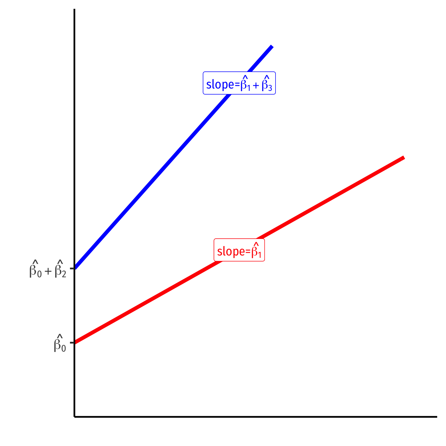
Di=0 group: Yi=^β0+^β1Xi
Di=1 group: Yi=(^β0+^β2)+(^β1+^β3)Xi
Interpretting Coefficients I
Yi=β0+β1Xi+β2Di+β3(Xi×Di)
- To interpret the coefficients, compare cases after changing X by ΔX:
Interpretting Coefficients I
Yi=β0+β1Xi+β2Di+β3(Xi×Di)
- To interpret the coefficients, compare cases after changing X by ΔX:
Yi+ΔYi=β0+β1(Xi+ΔXi)β2Di+β3((Xi+ΔXi)Di)
Interpretting Coefficients I
Yi=β0+β1Xi+β2Di+β3(Xi×Di)
- To interpret the coefficients, compare cases after changing X by ΔX:
Yi+ΔYi=β0+β1(Xi+ΔXi)β2Di+β3((Xi+ΔXi)Di)
- Subtracting these two equations, the difference is:
Interpretting Coefficients I
Yi=β0+β1Xi+β2Di+β3(Xi×Di)
- To interpret the coefficients, compare cases after changing X by ΔX:
Yi+ΔYi=β0+β1(Xi+ΔXi)β2Di+β3((Xi+ΔXi)Di)
- Subtracting these two equations, the difference is:
ΔYi=β1ΔXi+β3DiΔXiΔYiΔXi=β1+β3Di
Interpretting Coefficients I
Yi=β0+β1Xi+β2Di+β3(Xi×Di)
- To interpret the coefficients, compare cases after changing X by ΔX:
Yi+ΔYi=β0+β1(Xi+ΔXi)β2Di+β3((Xi+ΔXi)Di)
- Subtracting these two equations, the difference is:
ΔYi=β1ΔXi+β3DiΔXiΔYiΔXi=β1+β3Di
The effect of X→Y depends on the value of Di!
β3: increment to the effect of X→Y when Di=1 (vs. Di=0
Interpretting Coefficients II
Yi=β0+β1Xi+β2Di+β3(Xi×Di)
- ^β0: Yi for Xi=0 and Di=0
Interpretting Coefficients II
Yi=β0+β1Xi+β2Di+β3(Xi×Di)
^β0: Yi for Xi=0 and Di=0
β1: Marginal effect of Xi→Yi for Di=0
Interpretting Coefficients II
Yi=β0+β1Xi+β2Di+β3(Xi×Di)
^β0: Yi for Xi=0 and Di=0
β1: Marginal effect of Xi→Yi for Di=0
β2: Marginal effect on Yi of difference between Di=0 and Di=1
Interpretting Coefficients II
Yi=β0+β1Xi+β2Di+β3(Xi×Di)
^β0: Yi for Xi=0 and Di=0
β1: Marginal effect of Xi→Yi for Di=0
β2: Marginal effect on Yi of difference between Di=0 and Di=1
β3: The difference of the marginal effect of Xi→Yi between Di=0 and Di=1
Interpretting Coefficients II
Yi=β0+β1Xi+β2Di+β3(Xi×Di)
^β0: Yi for Xi=0 and Di=0
β1: Marginal effect of Xi→Yi for Di=0
β2: Marginal effect on Yi of difference between Di=0 and Di=1
β3: The difference of the marginal effect of Xi→Yi between Di=0 and Di=1
This is a bit awkward, easier to think about the two regression lines:
Interpretting Coefficients III
Yi=β0+β1Xi+β2Di+β3(Xi×Di)
- For Di=0 Group: ^Yi=^β0+^β1Xi
- Intercept (Yi for Xi=0): ^β0
- Slope (Marginal effect of Xi→Yi for Di=0 group): ^β1
Interpretting Coefficients III
Yi=β0+β1Xi+β2Di+β3(Xi×Di)
For Di=0 Group: ^Yi=^β0+^β1Xi
- Intercept (Yi for Xi=0): ^β0
- Slope (Marginal effect of Xi→Yi for Di=0 group): ^β1
For Di=1 Group: ^Yi=(^β0+^β2)+(^β1+^β3)Xi
- Intercept (Yi for Xi=0): ^β0+^β2
- Slope (Marginal effect of Xi→Yi for Di=1 group): ^β1+^β3
How can we determine if the two lines have the same slope and/or intercept?
- Same intercept? t-test H0: β2=0
- Same slope? t-test H0: β3=0
Example I
Example: ^wagei=^β0+^β1experi+^β2femalei+^β3(experi×femalei)
Example I
Example: ^wagei=^β0+^β1experi+^β2femalei+^β3(experi×femalei)
- For males (female=0):
^wagei=^β0+^β1exper
Example I
Example: ^wagei=^β0+^β1experi+^β2femalei+^β3(experi×femalei)
For males (female=0): ^wagei=^β0+^β1exper
For females (female=1): ^wagei=(^β0+^β2)⏟intercept+(^β1+^β3)⏟slopeexper
Example II
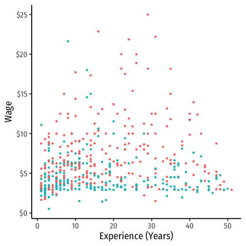
interaction_plot<-ggplot(data = wages)+ aes(x = exper, y = wage, color = as.factor(female))+ # make female factor geom_point()+ #geom_smooth(method = "lm")+ scale_y_continuous(labels=scales::dollar)+ labs(x = "Experience (Years)", y = "Wage")+ guides(color=F)+ # hide legend theme_classic(base_family = "Fira Sans Condensed", base_size=20)interaction_plot- Need to make sure
femaleis afactorvariable- Use
as.factor()in plot
- Use
Example II
interaction_plot+ geom_smooth(method="lm")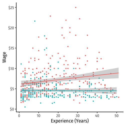
Example II
interaction_plot+ geom_smooth(method="lm", color = "black")+ facet_wrap(~female)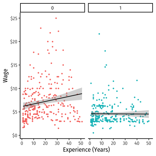
Example Regression in R I
- Syntax for an interaction term is easy in
R:var1:var2- Or could just do
var1*var2(multiply)
- Or could just do
Example Regression in R II
summary(interaction_reg)## ## Call:## lm(formula = wage ~ female + exper + female:exper, data = wages)## ## Residuals:## Min 1Q Median 3Q Max ## -6.3200 -1.8191 -0.9708 1.4132 17.2672 ## ## Coefficients:## Estimate Std. Error t value Pr(>|t|) ## (Intercept) 6.15828 0.34167 18.024 < 2e-16 ***## female -1.54655 0.48186 -3.210 0.001411 ** ## exper 0.05360 0.01544 3.472 0.000559 ***## female:exper -0.05507 0.02217 -2.483 0.013325 * ## ---## Signif. codes: 0 '***' 0.001 '**' 0.01 '*' 0.05 '.' 0.1 ' ' 1## ## Residual standard error: 3.443 on 522 degrees of freedom## Multiple R-squared: 0.1356, Adjusted R-squared: 0.1307 ## F-statistic: 27.31 on 3 and 522 DF, p-value: < 2.2e-16Example Regression in R III
library(huxtable)huxreg(interaction_reg, coefs = c("Constant" = "(Intercept)", "Experience" = "exper", "Female" = "female", "Female * Exper" = "female:exper"), statistics = c("N" = "nobs", "R-Squared" = "r.squared", "SER" = "sigma"), number_format = 2)| (1) | |
| Constant | 6.16 *** |
| (0.34) | |
| Experience | 0.05 *** |
| (0.02) | |
| Female | -1.55 ** |
| (0.48) | |
| Female * Exper | -0.06 * |
| (0.02) | |
| N | 526 |
| R-Squared | 0.14 |
| SER | 3.44 |
| *** p < 0.001; ** p < 0.01; * p < 0.05. | |
Example Regression in R: Interpretting Coefficients
^wagei=6.16+0.05Experiencei−1.55Femalei−0.06(Experiencei×Femalei)
Example Regression in R: Interpretting Coefficients
^wagei=6.16+0.05Experiencei−1.55Femalei−0.06(Experiencei×Femalei)
- ^β0:
Example Regression in R: Interpretting Coefficients
^wagei=6.16+0.05Experiencei−1.55Femalei−0.06(Experiencei×Femalei)
- ^β0: Men with experience of 0 years earn $6.16
Example Regression in R: Interpretting Coefficients
^wagei=6.16+0.05Experiencei−1.55Femalei−0.06(Experiencei×Femalei)
^β0: Men with experience of 0 years earn $6.16
^β1:
Example Regression in R: Interpretting Coefficients
^wagei=6.16+0.05Experiencei−1.55Femalei−0.06(Experiencei×Femalei)
^β0: Men with experience of 0 years earn $6.16
^β1: For every additional year of experience, men earn $0.05
Example Regression in R: Interpretting Coefficients
^wagei=6.16+0.05Experiencei−1.55Femalei−0.06(Experiencei×Femalei)
^β0: Men with experience of 0 years earn $6.16
^β1: For every additional year of experience, men earn $0.05
^β2:
Example Regression in R: Interpretting Coefficients
^wagei=6.16+0.05Experiencei−1.55Femalei−0.06(Experiencei×Femalei)
^β0: Men with experience of 0 years earn $6.16
^β1: For every additional year of experience, men earn $0.05
^β2: Women on average earn $1.55 less than men, holding experience constant
^β3:
Example Regression in R: Interpretting Coefficients
^wagei=6.16+0.05Experiencei−1.55Femalei−0.06(Experiencei×Femalei)
^β0: Men with experience of 0 years earn $6.16
^β1: For every additional year of experience, men earn $0.05
^β2: Women on average earn $1.55 less than men, holding experience constant
^β3: Women earn $0.06 less than men for every additional year of experience
Example Regression in R: Interpretting Coefficients as Two Regressions I
^wagei=6.16+0.05Experiencei−1.55Femalei−0.06(Experiencei×Femalei)
Example Regression in R: Interpretting Coefficients as Two Regressions I
^wagei=6.16+0.05Experiencei−1.55Femalei−0.06(Experiencei×Femalei)
Regression for men female=0) ^wagei=6.16+0.05Experience
Example Regression in R: Interpretting Coefficients as Two Regressions I
^wagei=6.16+0.05Experiencei−1.55Femalei−0.06(Experiencei×Femalei)
Regression for men female=0) ^wagei=6.16+0.05Experience
- Men with no experience earn $6.16
Example Regression in R: Interpretting Coefficients as Two Regressions I
^wagei=6.16+0.05Experiencei−1.55Femalei−0.06(Experiencei×Femalei)
Regression for men female=0) ^wagei=6.16+0.05Experience
Men with no experience earn $6.16
For every additional year of experience, men earn $0.05 more
Example Regression in R: Interpretting Coefficients as Two Regressions II
^wagei=6.16+0.05Experiencei−1.55Femalei−0.06(Experiencei×Femalei)
Regression for women female=1) ^wagei=6.16+0.05Experience−1.55(1)−0.06Experience×(1)=(6.16−1.55)+(0.05−0.06)Experience=4.61−0.01Experience
Example Regression in R: Interpretting Coefficients as Two Regressions II
^wagei=6.16+0.05Experiencei−1.55Femalei−0.06(Experiencei×Femalei)
Regression for women female=1) ^wagei=6.16+0.05Experience−1.55(1)−0.06Experience×(1)=(6.16−1.55)+(0.05−0.06)Experience=4.61−0.01Experience
- Women with no experience earn $4.61
Example Regression in R: Interpretting Coefficients as Two Regressions II
^wagei=6.16+0.05Experiencei−1.55Femalei−0.06(Experiencei×Femalei)
Regression for women female=1) ^wagei=6.16+0.05Experience−1.55(1)−0.06Experience×(1)=(6.16−1.55)+(0.05−0.06)Experience=4.61−0.01Experience
Women with no experience earn $4.61
For every additional year of experience, women earn $0.01 less
Example Regression in R: Hypothesis Testing
Test the significance of interaction effects
Think: are slopes and intercepts of the two regressions statistically significantly different?
Are intercepts different?
- Difference between men vs. women for no experience?
- Is ^β2 significant?
- Yes: t=−3.210, p-value = 0.00
Are slopes different?
- Difference between men vs. women for marginal effect of experience?
- Is ^β3 significant?
- Yes: t=−2.48, p-value = 0.01
library(broom)tidy(interaction_reg)| term | estimate | std.error | statistic | p.value |
| (Intercept) | 6.16 | 0.342 | 18 | 8e-57 |
| female | -1.55 | 0.482 | -3.21 | 0.00141 |
| exper | 0.0536 | 0.0154 | 3.47 | 0.000559 |
| female:exper | -0.0551 | 0.0222 | -2.48 | 0.0133 |
Interactions Between Two Dummy Variables
Interactions Between Two Dummy Variables
Yi=β0+β1D1i+β2D2i+β3(D1i×D2i)
- D1i and D2i are dummy variables
Interactions Between Two Dummy Variables
Yi=β0+β1D1i+β2D2i+β3(D1i×D2i)
D1i and D2i are dummy variables
^β1: effect on Y of going from D1i=0 to D1i=1 for D2i=0
Interactions Between Two Dummy Variables
Yi=β0+β1D1i+β2D2i+β3(D1i×D2i)
D1i and D2i are dummy variables
^β1: effect on Y of going from D1i=0 to D1i=1 for D2i=0
^β2: effect on Y of going from D2i=0 to D2i=1 for D1i=0
Interactions Between Two Dummy Variables
Yi=β0+β1D1i+β2D2i+β3(D1i×D2i)
D1i and D2i are dummy variables
^β1: effect on Y of going from D1i=0 to D1i=1 for D2i=0
^β2: effect on Y of going from D2i=0 to D2i=1 for D1i=0
^β3: effect on Y of going from D1i=0 and D2i=1 to D1i=1 and D2i=1
- increment to the effect of D1i going from 0 to 1 when D2i=1 (vs. 0)
- increment to the effect of D2i going from 0 to 1 when D1i=1 (vs. 0)
- As always, best to think logically about possibilities (when each dummy =0 or =1)
Interactions Between Two Dummy Variables: Interpretting Coefficients
Yi=β0+β1D1i+β2D2i+β3(D1i×D2i)
Interactions Between Two Dummy Variables: Interpretting Coefficients
Yi=β0+β1D1i+β2D2i+β3(D1i×D2i)
- To interpret coefficients, compare cases (for Di1 as an example):
E(Yi|D1i=0,D2i=d2)=β0+β2d2E(Yi|D1i=1,D2i=d2)=β0+β1(1)+β2d2+β3(1)d2
Interactions Between Two Dummy Variables: Interpretting Coefficients
Yi=β0+β1D1i+β2D2i+β3(D1i×D2i)
- To interpret coefficients, compare cases (for Di1 as an example):
E(Yi|D1i=0,D2i=d2)=β0+β2d2E(Yi|D1i=1,D2i=d2)=β0+β1(1)+β2d2+β3(1)d2
- Subtracting the two, the difference is:
β1+β3d2
- The effect of
\(D{1i} \rightarrow Y_i\)depends on the value of\(D{2i}\)- ^β3 is the increment to the effect of D1 on Y when D2=1
Interactions Between Two Dummy Variables: Example
Example: Does the gender pay gap change if a person is married vs. single?
^wagei=^β0+^β1femalei+^β2marriedi+^β3(femalei×marriedi)
Interactions Between Two Dummy Variables: Example
Example: Does the gender pay gap change if a person is married vs. single?
^wagei=^β0+^β1femalei+^β2marriedi+^β3(femalei×marriedi)
- Logically, there are 4 possible combinations of femalei={0,1} and marriedi={0,1}
Interactions Between Two Dummy Variables: Example
Example: Does the gender pay gap change if a person is married vs. single?
^wagei=^β0+^β1femalei+^β2marriedi+^β3(femalei×marriedi)
- Logically, there are 4 possible combinations of femalei={0,1} and marriedi={0,1}
- Unmarried men (femalei=0,marriedi=0)
^wagei=^β0
Interactions Between Two Dummy Variables: Example
Example: Does the gender pay gap change if a person is married vs. single?
^wagei=^β0+^β1femalei+^β2marriedi+^β3(femalei×marriedi)
- Logically, there are 4 possible combinations of femalei={0,1} and marriedi={0,1}
Unmarried men (femalei=0,marriedi=0) ^wagei=^β0
Married men (femalei=0,marriedi=1) ^wagei=^β0+^β2
Interactions Between Two Dummy Variables: Example
Example: Does the gender pay gap change if a person is married vs. single?
^wagei=^β0+^β1femalei+^β2marriedi+^β3(femalei×marriedi)
- Logically, there are 4 possible combinations of femalei={0,1} and marriedi={0,1}
- Unmarried women (femalei=1,marriedi=0)
^wagei=^β0+^β1
Interactions Between Two Dummy Variables: Example
Example: Does the gender pay gap change if a person is married vs. single?
^wagei=^β0+^β1femalei+^β2marriedi+^β3(femalei×marriedi)
- Logically, there are 4 possible combinations of femalei={0,1} and marriedi={0,1}
Unmarried women (femalei=1,marriedi=0) ^wagei=^β0+^β1
Married women (femalei=1,marriedi=1) ^wagei=^β0+^β1+^β2+^β3
Looking at the Data
# get average wage for unmarried menwages %>% filter(female == 0, married == 0) %>% summarize(mean = mean(wage))| mean |
| 5.17 |
# get average wage for married menwages %>% filter(female == 0, married == 1) %>% summarize(mean = mean(wage))| mean |
| 7.98 |
# get average wage for unmarried womenwages %>% filter(female == 1, married == 0) %>% summarize(mean = mean(wage))| mean |
| 4.61 |
# get average wage for married womenwages %>% filter(female == 1, married == 1) %>% summarize(mean = mean(wage))| mean |
| 4.57 |
Interactions Between Two Dummy Variables: Group Means
^wagei=^β0+^β1femalei+^β2marriedi+^β3(femalei×marriedi)
| Gender | Unmarried | Married |
|---|---|---|
| Male | $5.17 | $7.98 |
| Female | $4.61 | $4.57 |
Interactions Between Two Dummy Variables: In R I
reg_dummies<-lm(wage~female+married+female:married, data = wages)summary(reg_dummies)## ## Call:## lm(formula = wage ~ female + married + female:married, data = wages)## ## Residuals:## Min 1Q Median 3Q Max ## -5.7530 -1.7327 -0.9973 1.2566 17.0184 ## ## Coefficients:## Estimate Std. Error t value Pr(>|t|) ## (Intercept) 5.1680 0.3614 14.299 < 2e-16 ***## female -0.5564 0.4736 -1.175 0.241 ## married 2.8150 0.4363 6.451 2.53e-10 ***## female:married -2.8607 0.6076 -4.708 3.20e-06 ***## ---## Signif. codes: 0 '***' 0.001 '**' 0.01 '*' 0.05 '.' 0.1 ' ' 1## ## Residual standard error: 3.352 on 522 degrees of freedom## Multiple R-squared: 0.181, Adjusted R-squared: 0.1763 ## F-statistic: 38.45 on 3 and 522 DF, p-value: < 2.2e-16Interactions Between Two Dummy Variables: In R II
library(huxtable)huxreg(reg_dummies, coefs = c("Constant" = "(Intercept)", "Female" = "female", "Married" = "married", "Female * Married" = "female:married"), statistics = c("N" = "nobs", "R-Squared" = "r.squared", "SER" = "sigma"), number_format = 2)| (1) | |
| Constant | 5.17 *** |
| (0.36) | |
| Female | -0.56 |
| (0.47) | |
| Married | 2.82 *** |
| (0.44) | |
| Female * Married | -2.86 *** |
| (0.61) | |
| N | 526 |
| R-Squared | 0.18 |
| SER | 3.35 |
| *** p < 0.001; ** p < 0.01; * p < 0.05. | |
Interactions Between Two Dummy Variables: Interpretting Coefficients
^wagei=5.17−0.56femalei+2.82marriedi−2.86(femalei×marriedi)
| Gender | Unmarried | Married |
|---|---|---|
| Male | $5.17 | $7.98 |
| Female | $4.61 | $4.57 |
Interactions Between Two Dummy Variables: Interpretting Coefficients
^wagei=5.17−0.56femalei+2.82marriedi−2.86(femalei×marriedi)
| Gender | Unmarried | Married |
|---|---|---|
| Male | $5.17 | $7.98 |
| Female | $4.61 | $4.57 |
- Wage for unmarried men: ^β0=5.17
Interactions Between Two Dummy Variables: Interpretting Coefficients
^wagei=5.17−0.56femalei+2.82marriedi−2.86(femalei×marriedi)
| Gender | Unmarried | Married |
|---|---|---|
| Male | $5.17 | $7.98 |
| Female | $4.61 | $4.57 |
Wage for unmarried men: ^β0=5.17
Wage for married men: ^β0+^β2=5.17+2.82=7.98
Wage for unmarried women: ^β0+^β1=5.17−0.56=4.61
Wage for married women: ^β0+^β1+^β2+^β3=5.17−0.56+2.82−2.86=4.57
Interactions Between Two Continuous Variables
Interactions Between Two Continuous Variables
Yi=β0+β1X1i+β2X2i+β3(X1i×X2i)
Interactions Between Two Continuous Variables
Yi=β0+β1X1i+β2X2i+β3(X1i×X2i)
- To interpret coefficients, compare changes after changing ΔX1i:
Y+ΔY=β0+β1(X1+ΔX1)β2X2+β3((X1+ΔX1)×X2)
Interactions Between Two Continuous Variables
Yi=β0+β1X1i+β2X2i+β3(X1i×X2i)
- To interpret coefficients, compare changes after changing ΔX1i:
Y+ΔY=β0+β1(X1+ΔX1)β2X2+β3((X1+ΔX1)×X2)
- Take the difference to get:
Interactions Between Two Continuous Variables
Yi=β0+β1X1i+β2X2i+β3(X1i×X2i)
- To interpret coefficients, compare changes after changing ΔX1i:
Y+ΔY=β0+β1(X1+ΔX1)β2X2+β3((X1+ΔX1)×X2)
- Take the difference to get:
ΔY=β1ΔX1+β3X2ΔX1ΔYΔX1=β1+β3X2
Interactions Between Two Continuous Variables
Yi=β0+β1X1i+β2X2i+β3(X1i×X2i)
- To interpret coefficients, compare changes after changing ΔX1i:
Y+ΔY=β0+β1(X1+ΔX1)β2X2+β3((X1+ΔX1)×X2)
- Take the difference to get:
ΔY=β1ΔX1+β3X2ΔX1ΔYΔX1=β1+β3X2
The effect of X1→Yi depends on X2
β3: increment to the effect of X1→Yi from a 1 unit change in X2
Interactions Between Two Continuous Variables: Example
Example: Do education and experience interact in their determination of wages?
^wagei=^β0+^β1educi+^β2experi+^β3(educi×experi)
- Estimated effect of education on wages depends on the amount of experience (and vice versa)!
ΔwageΔeduc=^β1+β3exper
- This is a type of nonlinearity (we will examine nonlinearities next lesson)
Interactions Between Two Continuous Variables: In R I
reg_cont<-lm(wage~educ+exper+educ:exper, data = wages)summary(reg_cont)## ## Call:## lm(formula = wage ~ educ + exper + educ:exper, data = wages)## ## Residuals:## Min 1Q Median 3Q Max ## -5.6747 -1.9683 -0.6991 1.2803 15.8067 ## ## Coefficients:## Estimate Std. Error t value Pr(>|t|) ## (Intercept) -2.859916 1.181080 -2.421 0.0158 * ## educ 0.601735 0.089900 6.693 5.64e-11 ***## exper 0.045769 0.042614 1.074 0.2833 ## educ:exper 0.002062 0.003491 0.591 0.5549 ## ---## Signif. codes: 0 '***' 0.001 '**' 0.01 '*' 0.05 '.' 0.1 ' ' 1## ## Residual standard error: 3.259 on 522 degrees of freedom## Multiple R-squared: 0.2257, Adjusted R-squared: 0.2212 ## F-statistic: 50.71 on 3 and 522 DF, p-value: < 2.2e-16Interactions Between Two Continuous Variables: In R II
library(huxtable)huxreg(reg_cont, coefs = c("Constant" = "(Intercept)", "Education" = "educ", "Experience" = "exper", "Education * Experience" = "educ:exper"), statistics = c("N" = "nobs", "R-Squared" = "r.squared", "SER" = "sigma"), number_format = 3)| (1) | |
| Constant | -2.860 * |
| (1.181) | |
| Education | 0.602 *** |
| (0.090) | |
| Experience | 0.046 |
| (0.043) | |
| Education * Experience | 0.002 |
| (0.003) | |
| N | 526 |
| R-Squared | 0.226 |
| SER | 3.259 |
| *** p < 0.001; ** p < 0.01; * p < 0.05. | |
Interactions Between Two Continuous Variables: Interpretting Coefficients
^wagesi=−2.860+0.602educi+0.047experi+0.002(educi×experi)
Interactions Between Two Continuous Variables: Interpretting Coefficients
^wagesi=−2.860+0.602educi+0.047experi+0.002(educi×experi)
Changes in Education:
| Experience | ΔwageΔeduc |
|---|---|
| 5 years | 0.602+0.002(5)=0.612 |
| 10 years | 0.602+0.002(10)=0.622 |
| 15 years | 0.602+0.002(15)=0.632 |
- Marginal effect of education → wages increases with more experience (but very insignificantly)