3.3: Model Specification Strategies
ECON 480 · Econometrics · Fall 2019
Ryan Safner
Assistant Professor of Economics
safner@hood.edu
ryansafner/metricsf19
metricsF19.classes.ryansafner.com
Model Specification
The big challenge in applied econometrics is choosing how to specify a model to regress
Every dataset is different, every study has a different goal
- there is no bright line rule, only a set of guidelines and skills that you can only learn by doing!
But here are some helpful tips and frequent problems (and solutions)
Model Specification: Process
1. Identify your question of interest: what do you want to know? What marginal effect(s) do you want to estimate?
Model Specification: Process
1. Identify your question of interest: what do you want to know? What marginal effect(s) do you want to estimate?
2. Think about possible sources of endogeneity: what other variables would cause omitted variable bias if we left them out? Can we get data on them too?
- Again: must BOTH (1) affect Y AND (2) be correlated with X
- This requires much of your economic intuitions: R2 and statistical measures cannot tell you everything!
3. Run multiple models and check the robustness of your results: does the size (or direction) of your marginal effect(s) of interest change as you change your model (i.e. add more variables)?
4. Interpret your results
- Are they statistically significant?
- Regardless of statistical significance, are they economically meaningful?
- Why should we care?
- How big is "big"?
Proxy Variables
- Ideally, we would want a randomized control experiment to assign individuals to treatment
Proxy Variables
Ideally, we would want a randomized control experiment to assign individuals to treatment
But with observational data, ui depends on other factors
- If we can observe and measure these factors, then include them in the regression
Proxy Variables
Ideally, we would want a randomized control experiment to assign individuals to treatment
But with observational data, ui depends on other factors
- If we can observe and measure these factors, then include them in the regression
- If we can't directly measure them, often we can include variables correlated with these variables to proxy for the effects of them!
Proxy Variables: Example I
Example: Consider test scores and class sizes again. What about learning opportunities outside of school?
Proxy Variables: Example I
Example: Consider test scores and class sizes again. What about learning opportunities outside of school?
- Probably a bias-causing omitted variable (affects test score and correlated with class size) but we can't measure it!
Proxy Variables: Example I
Example: Consider test scores and class sizes again. What about learning opportunities outside of school?
Probably a bias-causing omitted variable (affects test score and correlated with class size) but we can't measure it!
Suppose we can measure a variable V, and significantly, corr(V,Z)≠0
- e.g. we have data on the percent of students who get a free or subsidized lunch (
meal_pct)
- e.g. we have data on the percent of students who get a free or subsidized lunch (
This is a good proxy for income-determined learning opportunities outside of school
meal_pctis correlated with Income (which is likely correlated with both class size and test score)- A good indirect measure of Income
Proxy Variables: Example II
- We assumed we don't have data on average district income, we would expect
meal_pctto be strongly negatively correlated with income
Proxy Variables: Example II
We assumed we don't have data on average district income, we would expect
meal_pctto be strongly negatively correlated with incomeJust kidding, we do have data on
avginc, but we'll only use it to confirm our suspicion:
Proxy Variables: Example II
We assumed we don't have data on average district income, we would expect
meal_pctto be strongly negatively correlated with incomeJust kidding, we do have data on
avginc, but we'll only use it to confirm our suspicion:
CASchool %>% select(testscr, str, el_pct, avginc,meal_pct) %>% cor()## testscr str el_pct avginc meal_pct## testscr 1.0000000 -0.2263628 -0.6441237 0.7124308 -0.8687720## str -0.2263628 1.0000000 0.1876424 -0.2321937 0.1352034## el_pct -0.6441237 0.1876424 1.0000000 -0.3074195 0.6530607## avginc 0.7124308 -0.2321937 -0.3074195 1.0000000 -0.6844396## meal_pct -0.8687720 0.1352034 0.6530607 -0.6844396 1.0000000Proxy Variables: Example II
We assumed we don't have data on average district income, we would expect
meal_pctto be strongly negatively correlated with incomeJust kidding, we do have data on
avginc, but we'll only use it to confirm our suspicion:
CASchool %>% select(testscr, str, el_pct, avginc,meal_pct) %>% cor()## testscr str el_pct avginc meal_pct## testscr 1.0000000 -0.2263628 -0.6441237 0.7124308 -0.8687720## str -0.2263628 1.0000000 0.1876424 -0.2321937 0.1352034## el_pct -0.6441237 0.1876424 1.0000000 -0.3074195 0.6530607## avginc 0.7124308 -0.2321937 -0.3074195 1.0000000 -0.6844396## meal_pct -0.8687720 0.1352034 0.6530607 -0.6844396 1.0000000- We can see
meal_pctis strongly (negatively) correlated with income, as expected
Proxy Variables: Example III
proxyreg<-lm(testscr~str+el_pct+meal_pct, data=CASchool)summary(proxyreg)## ## Call:## lm(formula = testscr ~ str + el_pct + meal_pct, data = CASchool)## ## Residuals:## Min 1Q Median 3Q Max ## -32.849 -5.151 -0.308 5.243 31.501 ## ## Coefficients:## Estimate Std. Error t value Pr(>|t|) ## (Intercept) 700.14996 4.68569 149.423 < 2e-16 ***## str -0.99831 0.23875 -4.181 3.54e-05 ***## el_pct -0.12157 0.03232 -3.762 0.000193 ***## meal_pct -0.54735 0.02160 -25.341 < 2e-16 ***## ---## Signif. codes: 0 '***' 0.001 '**' 0.01 '*' 0.05 '.' 0.1 ' ' 1## ## Residual standard error: 9.08 on 416 degrees of freedom## Multiple R-squared: 0.7745, Adjusted R-squared: 0.7729 ## F-statistic: 476.3 on 3 and 416 DF, p-value: < 2.2e-16Interpreting Control Variables
^Test Scorei=700.15−1.00STRi−0.122%ELi−0.547meal%i
Interpreting Control Variables
^Test Scorei=700.15−1.00STRi−0.122%ELi−0.547meal%i
- Is
meal%causal?
Interpreting Control Variables
^Test Scorei=700.15−1.00STRi−0.122%ELi−0.547meal%i
Is
meal%causal?Getting rid of programs in districts where a large percentage of students need them would boost test scores A LOT! (So probably not causal...)
Interpreting Control Variables
^Test Scorei=700.15−1.00STRi−0.122%ELi−0.547meal%i
Is
meal%causal?Getting rid of programs in districts where a large percentage of students need them would boost test scores A LOT! (So probably not causal...)
meal%likely correlated with other things in ui (like outside learning opportunities!).- In fact, that's exactly why we included it as a variable!
- We don't need the OLS estimate on
meal%to be unbiased!- We only care about getting the estimate on
strto be unbiased!
- We only care about getting the estimate on
Control Variables
- A control variable is a regressor variable note of interest, but included to hold factors constant that, if omitted, would bias the causal effect of interest
Control Variables
A control variable is a regressor variable note of interest, but included to hold factors constant that, if omitted, would bias the causal effect of interest
The control variable may still be correlated with omitted causal factors in u
- Estimators (ˆβ's) on control variables can be biased and that is OK!
- So long as we have unbiased estimators (ˆβ's) on the regressors we do care about!
- Control variables allow us to proceed as if X were randomly assigned
Coefficient Plots I
- Sometimes it is helpful to make a coefficient plot to visualize the different marginal effects
Coefficient Plots I
Sometimes it is helpful to make a coefficient plot to visualize the different marginal effects
Take
broomandtidy()your regression withconf.int=TRUE(and save as an object)
# run regressionreg<-lm(testscr~str+el_pct+meal_pct, data=CASchool)# load broomlibrary(broom)# tidy regression with confidence intervals# save as "reg_tidy"reg_tidy <- tidy(reg, conf.int = TRUE)Coefficient Plots II
# look at itreg_tidy| ABCDEFGHIJ0123456789 |
term <chr> | estimate <dbl> | std.error <dbl> | statistic <dbl> | p.value <dbl> | conf.low <dbl> | conf.high <dbl> |
|---|---|---|---|---|---|---|
| (Intercept) | 700.1499647 | 4.68568657 | 149.423132 | 0.000000e+00 | 690.9393907 | 709.36053869 |
| str | -0.9983092 | 0.23875427 | -4.181325 | 3.535856e-05 | -1.4676244 | -0.52899403 |
| el_pct | -0.1215733 | 0.03231728 | -3.761867 | 1.928408e-04 | -0.1850988 | -0.05804777 |
| meal_pct | -0.5473456 | 0.02159885 | -25.341424 | 2.302903e-86 | -0.5898020 | -0.50488907 |
# intercept is too big relative to others! let's leave it outreg_tidy_no_int<-reg_tidy %>% filter(term!="(Intercept)")Coefficient Plots III
ggplot(data = reg_tidy_no_int)+ aes(x = estimate, y = term, color = term)+ geom_point()+ # point for estimate # now make "error bars" using conf. int. geom_segment(aes(x = conf.low, xend = conf.high, y=term, yend=term))+ # add line at 0 geom_vline(xintercept=0, size=1, color="black", linetype="dashed")+ scale_x_continuous(breaks=seq(-1.5,0.5,0.5), limits=c(-1.5,0.5))+ labs(x = expression(paste("Marginal effect, ", hat(beta[j]))), y = "Variable")+ guides(color=F)+ # hide legend theme_classic(base_family = "Fira Sans Condensed", base_size=20)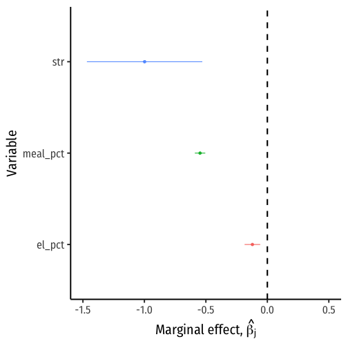
Model Specification Warning: R2
Do NOT just try to maximize R2 or ˉR2
A high R2 or ˉR2 means that the regressors explain variation in Y
A high R2 or ˉR2 does NOT mean you have eliminated omitted variable bias
A high R2 or ˉR2 does NOT mean you have an unbiased estimate of a causal effect
A high R2 or ˉR2 does NOT mean included variables are statistically significant
Model Specification: Goal
We care mostly about measuring a causal effect
This involves making the respective ^βj's as unbiased as possible (because βj is the causal effect of Xj→Y!
You will not get high R2's in social science
- even if you do, you are only explaining variation in Y with the model, not necessarily the causal effect!