3.2: Multivariate OLS Estimators: Bias, Precision, and Fit
ECON 480 · Econometrics · Fall 2019
Ryan Safner
Assistant Professor of Economics
safner@hood.edu
ryansafner/metricsf19
metricsF19.classes.ryansafner.com
The Multivariate OLS Estimators
The Multivariate OLS Estimators
- By analogy, we still focus on the ordinary least squares (OLS) estimators of the unknown population parameters β0,β1,β2,⋯,βk which solves:
min^β0,^β1,^β2,⋯,^βkn∑i=1[Yi−(^β0+^β1X1i+^β2X2i+⋯+^βkXki)⏟ui]2
- Again, OLS estimators are chosen to minimize the sum of squared errors (SSE)
- i.e. the sum of the squared distances between the actual values of Yi and the predicted values ^Yi
The Multivariate OLS Estimators: FYI
Math FYI: in linear algebra terms, a regression model with n observations of k independent variables:
Y=Xβ+u
(y1y2⋮yn)⏟Y(n×1)=(x1,1x1,2⋯x1,nx2,1x2,2⋯x2,n⋮⋮⋱⋮xk,1xk,2⋯xk,n)⏟X(n×k)(β1β2⋮βk)⏟β(k×1)+(u1u2⋮un)⏟u(n×1)
The Multivariate OLS Estimators: FYI
Math FYI: in linear algebra terms, a regression model with n observations of k independent variables:
Y=Xβ+u
(y1y2⋮yn)⏟Y(n×1)=(x1,1x1,2⋯x1,nx2,1x2,2⋯x2,n⋮⋮⋱⋮xk,1xk,2⋯xk,n)⏟X(n×k)(β1β2⋮βk)⏟β(k×1)+(u1u2⋮un)⏟u(n×1)
- The OLS estimator for β is ˆβ=(X′X)−1X′Y
The Multivariate OLS Estimators: FYI
Math FYI: in linear algebra terms, a regression model with n observations of k independent variables:
Y=Xβ+u
(y1y2⋮yn)⏟Y(n×1)=(x1,1x1,2⋯x1,nx2,1x2,2⋯x2,n⋮⋮⋱⋮xk,1xk,2⋯xk,n)⏟X(n×k)(β1β2⋮βk)⏟β(k×1)+(u1u2⋮un)⏟u(n×1)
The OLS estimator for β is ˆβ=(X′X)−1X′Y
Appreciate that I am saving you from such sorrow
The Sampling Distribution of ^βj
The Sampling Distribution of ^βj I
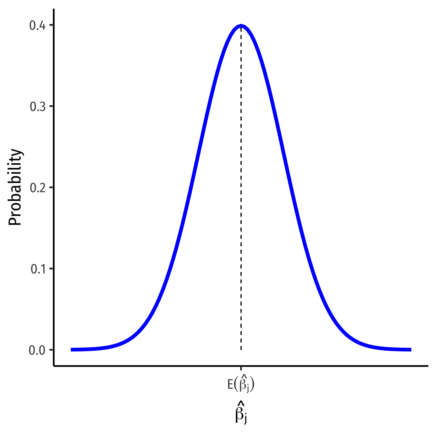
- For any individual βj, it has a sampling distribution:
^βj∼N(E[^βj],se(^βj))
- We want to know its sampling distribution's:
- Center: E[^βj]; what is the expected value of our estimator?
- Spread: se(^βj); how precise is our estimator?
The Expected Value of ^βj: Bias
Exogeneity and Unbiasedness
As before, E[^βj]=βj when Xj is exogenous (i.e. cor(Xj,u)=0)
We know the true E[^βj]=βj+cor(Xj,u)σuσXj⏟O.V. Bias
If Xj is endogenous (i.e. cor(Xj,u)≠0), contains omitted variable bias
We can now try to quantify the omitted variable bias
Measuring Omitted Variable Bias I
- Suppose the true population model of a relationship is:
Yi=β0+β1X1i+β2X2i+ui
- What happens when we run a regression and omit X2i?
Measuring Omitted Variable Bias I
- Suppose the true population model of a relationship is:
Yi=β0+β1X1i+β2X2i+ui
What happens when we run a regression and omit X2i?
Suppose we estimate the following omitted regression of just Yi on X1i (omitting X2i):+
Yi=α0+α1X1i+νi
+ Note: I am using α's and νi only to denote these are different estimates than the true model β's and ui
Measuring Omitted Variable Bias II
- Key Question: are X1i and X2i correlated?
Measuring Omitted Variable Bias II
Key Question: are X1i and X2i correlated?
Run an auxiliary regression of X2i on X1i to see:+
X2i=δ0+δ1X1i+τi
Measuring Omitted Variable Bias II
Key Question: are X1i and X2i correlated?
Run an auxiliary regression of X2i on X1i to see:+
X2i=δ0+δ1X1i+τi
If δ1=0, then X1i and X2i are not linearly related
If |δ1| is very big, then X1i and X2i are strongly linearly related
+ Note: I am using δ's and τ to differentiate estimates for this model.
Measuring Omitted Variable Bias III
- Now substitute our auxiliary regression between X2i and X1i into the true model:
- We know X2i=δ0+δ1X1i+τi
Yi=β0+β1X1i+β2X2i+ui
Measuring Omitted Variable Bias III
- Now substitute our auxiliary regression between X2i and X1i into the true model:
- We know X2i=δ0+δ1X1i+τi
Yi=β0+β1X1i+β2X2i+uiYi=β0+β1X1i+β2(δ0+δ1X1i+τi)+ui
Measuring Omitted Variable Bias III
- Now substitute our auxiliary regression between X2i and X1i into the true model:
- We know X2i=δ0+δ1X1i+τi
Yi=β0+β1X1i+β2X2i+uiYi=β0+β1X1i+β2(δ0+δ1X1i+τi)+uiYi=(β0+β2δ0)+(β1+β2δ1)X1i+(β2τi+ui)
Measuring Omitted Variable Bias III
- Now substitute our auxiliary regression between X2i and X1i into the true model:
- We know X2i=δ0+δ1X1i+τi
Yi=β0+β1X1i+β2X2i+uiYi=β0+β1X1i+β2(δ0+δ1X1i+τi)+uiYi=(β0+β2δ0⏟α0)+(β1+β2δ1⏟α1)X1i+(β2τi+ui⏟νi)
- Now relabel each of the three terms as the OLS estimates (α's) and error (νi) from the omitted regression, so we again have:
Yi=α0+α1X1i+νi
- Crucially, this means that our OLS estimate for X1i in the omitted regression is:
α1=β1+β2δ1
Measuring Omitted Variable Bias IV
α1=β1 + β2δ1
- The Omitted Regression OLS estimate for X1i picks up both:
The true effect of X1 on Yi: (β1)
The true effect of X2 on Yi: (β2)
- As pulled through the relationship between X1 and X2: (δ1)
Measuring Omitted Variable Bias IV
α1=β1 + β2δ1
- The Omitted Regression OLS estimate for X1i picks up both:
The true effect of X1 on Yi: (β1)
The true effect of X2 on Yi: (β2)
- As pulled through the relationship between X1 and X2: (δ1)
- Recall our conditions for omitted variable bias from some variable Zi:
Zi must be a determinant of Yi ⟹ β2≠0
Zi must be correlated with Xi ⟹ δ1≠0
- Otherwise, if Zi does not fit these conditions, α1=β1 and the omitted regression is unbiased!
Measuring Omitted Variable Bias in Our Class Size Example I
## ## Call:## lm(formula = testscr ~ str + el_pct, data = CASchool)## ## Residuals:## Min 1Q Median 3Q Max ## -48.845 -10.240 -0.308 9.815 43.461 ## ## Coefficients:## Estimate Std. Error t value Pr(>|t|) ## (Intercept) 686.03225 7.41131 92.566 < 2e-16 ***## str -1.10130 0.38028 -2.896 0.00398 ** ## el_pct -0.64978 0.03934 -16.516 < 2e-16 ***## ---## Signif. codes: 0 '***' 0.001 '**' 0.01 '*' 0.05 '.' 0.1 ' ' 1## ## Residual standard error: 14.46 on 417 degrees of freedom## Multiple R-squared: 0.4264, Adjusted R-squared: 0.4237 ## F-statistic: 155 on 2 and 417 DF, p-value: < 2.2e-16- The "True" Regression (Yi on X1i and X2i)
^Test Scorei=686.03−1.10 STRi−0.65 %ELi
Measuring Omitted Variable Bias in Our Class Size Example II
## ## Call:## lm(formula = testscr ~ str, data = CASchool)## ## Residuals:## Min 1Q Median 3Q Max ## -47.727 -14.251 0.483 12.822 48.540 ## ## Coefficients:## Estimate Std. Error t value Pr(>|t|) ## (Intercept) 698.9330 9.4675 73.825 < 2e-16 ***## str -2.2798 0.4798 -4.751 2.78e-06 ***## ---## Signif. codes: 0 '***' 0.001 '**' 0.01 '*' 0.05 '.' 0.1 ' ' 1## ## Residual standard error: 18.58 on 418 degrees of freedom## Multiple R-squared: 0.05124, Adjusted R-squared: 0.04897 ## F-statistic: 22.58 on 1 and 418 DF, p-value: 2.783e-06- The "Omitted" Regression (Yi on just X1i)
^Test Scorei=698.93−2.28 STRi
Measuring Omitted Variable Bias in Our Class Size Example III
## ## Call:## lm(formula = el_pct ~ str, data = CASchool)## ## Residuals:## Min 1Q Median 3Q Max ## -20.823 -13.006 -6.849 7.834 74.601 ## ## Coefficients:## Estimate Std. Error t value Pr(>|t|) ## (Intercept) -19.8541 9.1626 -2.167 0.03081 * ## str 1.8137 0.4644 3.906 0.00011 ***## ---## Signif. codes: 0 '***' 0.001 '**' 0.01 '*' 0.05 '.' 0.1 ' ' 1## ## Residual standard error: 17.98 on 418 degrees of freedom## Multiple R-squared: 0.03521, Adjusted R-squared: 0.0329 ## F-statistic: 15.25 on 1 and 418 DF, p-value: 0.0001095- The "Auxiliary" Regression (X2i on X1i)
^%ELi=−19.85+1.81 STRi
Measuring Omitted Variable Bias in Our Class Size Example IV
"True" Regression
^Test Scorei=686.03−1.10 STRi−0.65 %EL
"Omitted" Regression
^Test Scorei=698.93 −2.28 STRi
"Auxiliary" Regression
^%ELi=−19.85+1.81 STRi
- Omitted Regression estimate for α1 on STR is −2.28
Measuring Omitted Variable Bias in Our Class Size Example IV
"True" Regression
^Test Scorei=686.03 −1.10 STRi−0.65 %EL
"Omitted" Regression
^Test Scorei=698.93 −2.28 STRi
"Auxiliary" Regression
^%ELi=−19.85+1.81 STRi
- Omitted Regression estimate for α1 on STR is −2.28
α1=β1 + β2δ1
- The true effect of STR on Test Score: -1.10
Measuring Omitted Variable Bias in Our Class Size Example IV
"True" Regression
^Test Scorei=686.03 −1.10 STRi −0.65 %EL
"Omitted" Regression
^Test Scorei=698.93 −2.28 STRi
"Auxiliary" Regression
^%ELi=−19.85+1.81 STRi
- Omitted Regression estimate for α1 on STR is −2.28
α1=β1 + β2δ1
The true effect of STR on Test Score: -1.10
The true effect of %EL on Test Score: -0.65
Measuring Omitted Variable Bias in Our Class Size Example IV
"True" Regression
^Test Scorei=686.03 −1.10 STRi −0.65 %EL
"Omitted" Regression
^Test Scorei=698.93 −2.28 STRi
"Auxiliary" Regression
^%ELi=−19.85+ 1.81 STRi
- Omitted Regression estimate for α1 on STR is −2.28
α1=β1 + β2δ1
The true effect of STR on Test Score: -1.10
The true effect of %EL on Test Score: -0.65
The relationship between STR and %EL: 1.81
So, for the omitted regression:
α1=−2.28 =−1.10 + −0.65 ( 1.81 )
- The bias is ( −0.65 )( 1.81 )=−1.18
Precision of ^βj
Precision of ^βj I
- σ^βj; how precise are our estimates? (today)
- Variance σ2^βj or standard error σ^βj
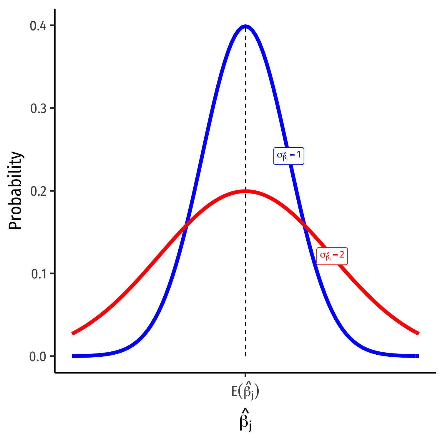
Precision of ^βj II
var(^βj)=11−R2j⏟VIF×(SER)2n×var(X)
se(^βj)=√var(^β1)
- Variation in ^βj is affected by four things now:
- Goodness of fit of the model (SER)
- Larger SER → larger var(^βj)
- Sample size, n
- Larger n → smaller var(^βj)
- Variance of X
- Larger var(X) → smaller var(^βj)
- Variance Inflation Factor 1(1−R2j)
- Larger VIF, larger var(^βj)
- This is the only new effect, explained in a moment
+ See Class 2.5 for a reminder of variation with just variable.
VIF and Multicollinearity I
- Two independent variables are multicollinear:
cor(Xj,Xl)≠0∀j≠l
VIF and Multicollinearity I
- Two independent variables are multicollinear:
cor(Xj,Xl)≠0∀j≠l
- Multicollinearity between X variables does not bias OLS estimates
- Remember, we pulled another variable out of u into the regression
- If it were omitted, then it would cause omitted variable bias!
VIF and Multicollinearity I
- Two independent variables are multicollinear:
cor(Xj,Xl)≠0∀j≠l
Multicollinearity between X variables does not bias OLS estimates
- Remember, we pulled another variable out of u into the regression
- If it were omitted, then it would cause omitted variable bias!
Multicollinearity does increase the variance of an estimate by
VIF=1(1−R2j)
VIF and Multicollinearity II
VIF=1(1−R2j)
- R2j is the R2 from an auxiliary regression of Xj on all other regressors (X's)
VIF and Multicollinearity II
VIF=1(1−R2j)
- R2j is the R2 from an auxiliary regression of Xj on all other regressors (X's)
Example: Suppose we have a regression with three regressors (k=3):
Yi=β0+β1X1i+β2X2i+β3X3i
VIF and Multicollinearity II
VIF=1(1−R2j)
- R2j is the R2 from an auxiliary regression of Xj on all other regressors (X's)
Example: Suppose we have a regression with three regressors (k=3):
Yi=β0+β1X1i+β2X2i+β3X3i
- There will be three different R2j's, one for each regressor:
R21 for X1i=γ+γX2i+γX3iR22 for X2i=ζ0+ζ1X1i+ζ2X3iR23 for X3i=η0+η1X1i+η2X2i
VIF and Multicollinearity III
VIF=1(1−R2j)
R2j is the R2 from an auxiliary regression of Xj on all other regressors (X's)
The R2j tells us how much other regressors explain regressor Xj
Key Takeaway: If other X variables explain Xj well (high R2J), it will be harder to tell how cleanly Xj→Yi, and so var(^βj) will be higher
VIF and Multicollinearity IV
- Common to calculate the Variance Inflation Factor (VIF) for each regressor:
VIF=1(1−R2j)
- VIF quantifies the factor (scalar) by which var(^βj) increases because of multicollinearity
- e.g. increases 2x, 3x, etc.
VIF and Multicollinearity IV
- Common to calculate the Variance Inflation Factor (VIF) for each regressor:
VIF=1(1−R2j)
- VIF quantifies the factor (scalar) by which var(^βj) increases because of multicollinearity
- e.g. increases 2x, 3x, etc.
- Baseline: R2j=0 ⟹ no multicollinearity ⟹ VIF = 1 (no inflation)
VIF and Multicollinearity IV
- Common to calculate the Variance Inflation Factor (VIF) for each regressor:
VIF=1(1−R2j)
- VIF quantifies the factor (scalar) by which var(^βj) increases because of multicollinearity
- e.g. increases 2x, 3x, etc.
Baseline: R2j=0 ⟹ no multicollinearity ⟹ VIF = 1 (no inflation)
Larger R2j ⟹ larger VIF
- Rule of thumb: VIF>10 is worrisome
VIF and Multicollinearity V
ggplot(data=CASchool, aes(x=str,y=el_pct))+ geom_point(color="blue")+ geom_smooth(method="lm", color="red")+ labs(x = "Student to Teacher Ratio", y = "Percentage of ESL Students")+ theme_classic(base_family = "Fira Sans Condensed", base_size=20)CAcorr_ex<-subset(CASchool, select=c("testscr", "str", "el_pct"))# Make a correlation tablecor(CAcorr_ex)## testscr str el_pct## testscr 1.0000000 -0.2263628 -0.6441237## str -0.2263628 1.0000000 0.1876424## el_pct -0.6441237 0.1876424 1.0000000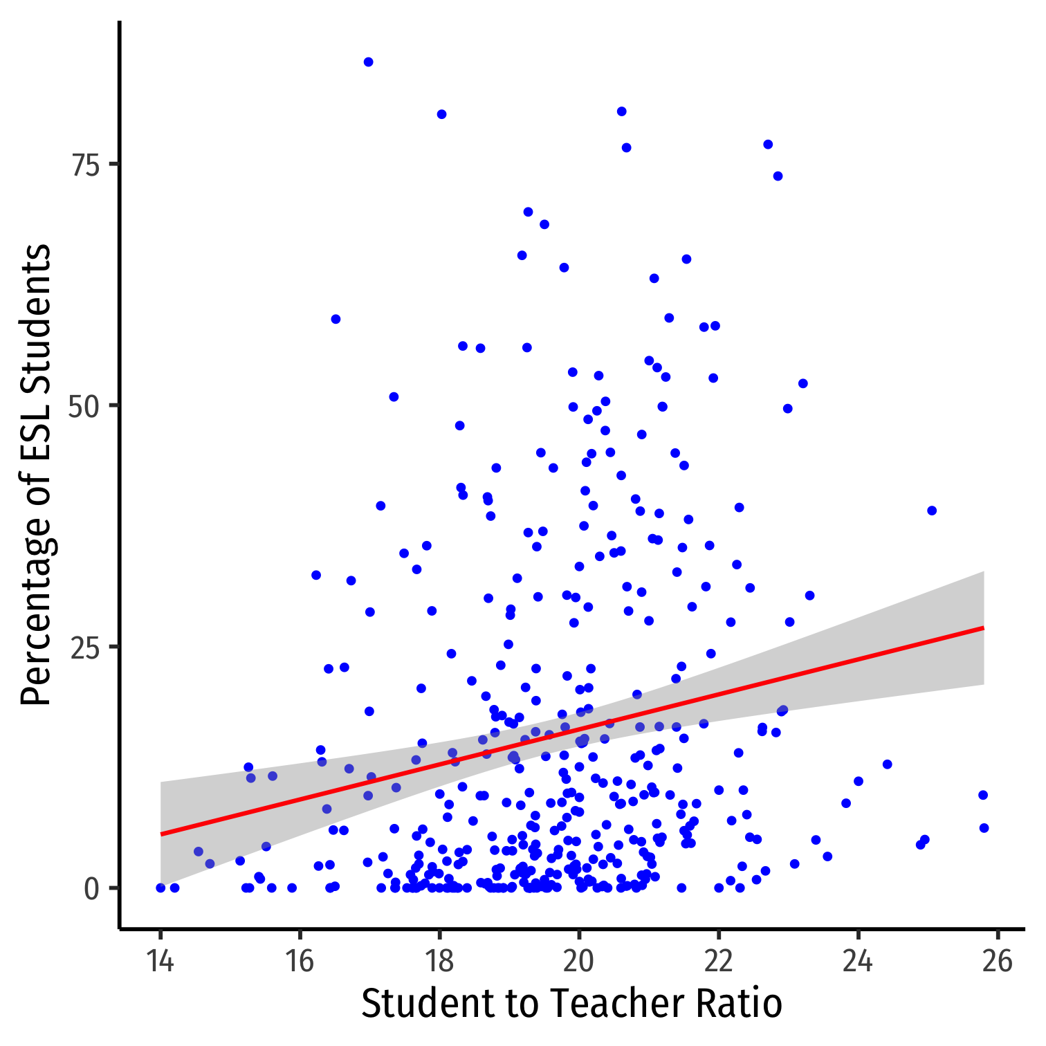
VIF and Multicollinearity in R I
# our multivariate regressionelreg<-lm(testscr~str+el_pct,data=CASchool)# use the "car" package for VIF function library("car") # syntax: vif(lm.object)vif(elreg)## str el_pct ## 1.036495 1.036495VIF and Multicollinearity in R I
# our multivariate regressionelreg<-lm(testscr~str+el_pct,data=CASchool)# use the "car" package for VIF function library("car") # syntax: vif(lm.object)vif(elreg)## str el_pct ## 1.036495 1.036495- var(^β1) on
strincreases by 1.036 times due to multicollinearity withel_pct - var(^β2) on
el_pctincreases by 1.036 times due to multicollinearity withstr
VIF and Multicollinearity in R II
- Let's calculate VIF manually to see where it comes from:
VIF and Multicollinearity in R II
- Let's calculate VIF manually to see where it comes from:
# run auxiliary regression of x2 on x1auxreg<-lm(el_pct~str, data=CASchool)# use broom package's tidy() command (cleaner)library(broom) # load broomtidy(auxreg) # look at reg output| ABCDEFGHIJ0123456789 |
term <chr> | estimate <dbl> | std.error <dbl> | statistic <dbl> | p.value <dbl> |
|---|---|---|---|---|
| (Intercept) | -19.854055 | 9.1626044 | -2.166857 | 0.0308099863 |
| str | 1.813719 | 0.4643735 | 3.905733 | 0.0001095165 |
VIF and Multicollinearity in R III
glance(auxreg) # look at aux reg stats for R^2| ABCDEFGHIJ0123456789 |
r.squared <dbl> | adj.r.squared <dbl> | sigma <dbl> | statistic <dbl> | p.value <dbl> | df <int> | logLik <dbl> | AIC <dbl> | |
|---|---|---|---|---|---|---|---|---|
| 0.03520966 | 0.03290155 | 17.98259 | 15.25475 | 0.0001095165 | 2 | -1808.502 | 3623.003 |
# extract our R-squared from aux regression (R_j^2)aux_r_squared<-glance(auxreg) %>% pull(r.squared)aux_r_squared # look at it## [1] 0.03520966VIF and Multicollinearity in R IV
# calculate VIF manuallyour_vif<-1/(1-aux_r_squared) # VIF formula our_vif## [1] 1.036495- Again, multicollinearity between the two X variables inflates the variance on each by 1.036 times
VIF and Multicollinearity: Another Example I
Example: For our Test Scores and Class Size example, what about district expenditures per student?
CAcorr2<-subset(CASchool, select=c("testscr", "str", "expn_stu"))# Make a correlation tablecorr2<-cor(CAcorr2)# look at itcorr2## testscr str expn_stu## testscr 1.0000000 -0.2263628 0.1912728## str -0.2263628 1.0000000 -0.6199821## expn_stu 0.1912728 -0.6199821 1.0000000VIF and Multicollinearity: Another Example II
ggplot(data=CASchool, aes(x=str,y=expn_stu))+ geom_point(color="blue")+ geom_smooth(method="lm", color="red")+ scale_y_continuous(labels = scales::dollar)+ labs(x = "Student to Teacher Ratio", y = "Expenditures per Student ($)")+ theme_classic(base_family = "Fira Sans Condensed", base_size=20)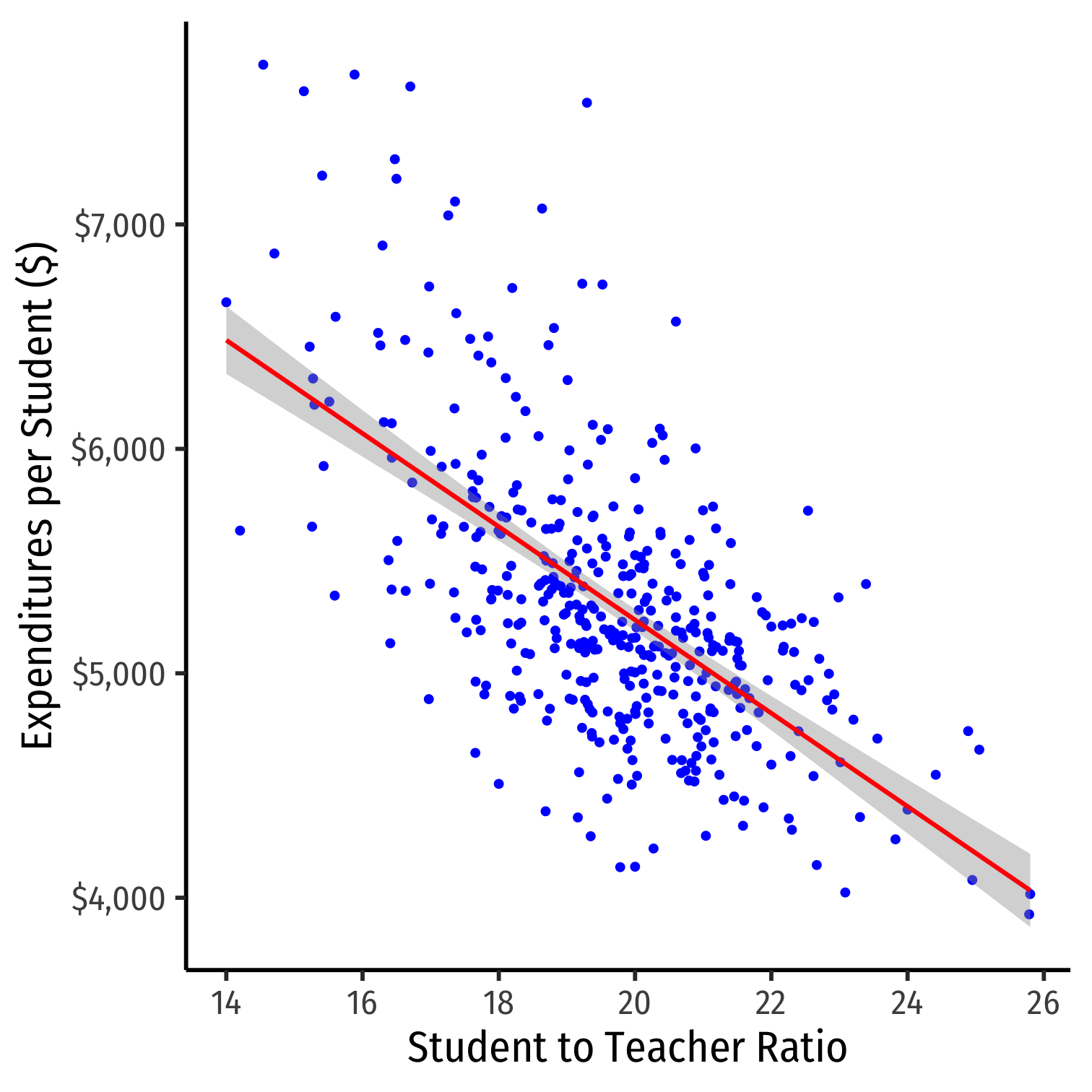
VIF and Multicollinearity: Another Example III
cor(Test score, expn)≠0
cor(STR, expn)≠0
VIF and Multicollinearity: Another Example III
cor(Test score, expn)≠0
cor(STR, expn)≠0
- Omitting expn will bias ^β1 on STR
VIF and Multicollinearity: Another Example III
cor(Test score, expn)≠0
cor(STR, expn)≠0
Omitting expn will bias ^β1 on STR
Including expn will not bias ^β1 on STR, but will make it less precise (higher variance)
VIF and Multicollinearity: Another Example III
cor(Test score, expn)≠0
cor(STR, expn)≠0
Omitting expn will bias ^β1 on STR
Including expn will not bias ^β1 on STR, but will make it less precise (higher variance)
Data tells us little about the effect of a change in STR holding expn constant
- Hard to know what happens to test scores when high STR AND high expn and vice versa (they rarely happen simultaneously)!
VIF and Multicollinearity: Another Example IV
expreg<-lm(testscr~str+expn_stu, data=CASchool)summary(expreg)## ## Call:## lm(formula = testscr ~ str + expn_stu, data = CASchool)## ## Residuals:## Min 1Q Median 3Q Max ## -47.507 -14.403 0.407 13.195 48.392 ## ## Coefficients:## Estimate Std. Error t value Pr(>|t|) ## (Intercept) 675.577174 19.562222 34.535 <2e-16 ***## str -1.763216 0.610914 -2.886 0.0041 ** ## expn_stu 0.002487 0.001823 1.364 0.1733 ## ---## Signif. codes: 0 '***' 0.001 '**' 0.01 '*' 0.05 '.' 0.1 ' ' 1## ## Residual standard error: 18.56 on 417 degrees of freedom## Multiple R-squared: 0.05545, Adjusted R-squared: 0.05092 ## F-statistic: 12.24 on 2 and 417 DF, p-value: 6.824e-06vif(expreg)## str expn_stu ## 1.624373 1.624373- Including
expn_stuincreases variance of ^β1 by 1.62 times
Multicollinearity Increases Variance
library(huxtable)huxreg("Model 1" = school_reg, "Model 2" = expreg, coefs = c("Intercept" = "(Intercept)", "Class Size" = "str", "Expenditures per Student" = "expn_stu"), statistics = c("N" = "nobs", "R-Squared" = "r.squared", "SER" = "sigma"), number_format = 2)- We can see SE(^β1) on
strincreases from 0.48 to 0.61 when we addexpn_stu
| Model 1 | Model 2 | |
| Intercept | 698.93 *** | 675.58 *** |
| (9.47) | (19.56) | |
| Class Size | -2.28 *** | -1.76 ** |
| (0.48) | (0.61) | |
| Expenditures per Student | 0.00 | |
| (0.00) | ||
| N | 420 | 420 |
| R-Squared | 0.05 | 0.06 |
| SER | 18.58 | 18.56 |
| *** p < 0.001; ** p < 0.01; * p < 0.05. | ||
Perfect Multicollinearity
- Perfect multicollinearity is when a regressor is an exact linear function of (an)other regressor(s)
Perfect Multicollinearity
- Perfect multicollinearity is when a regressor is an exact linear function of (an)other regressor(s)
^Sales=^β0+^β1Temperature (C)+^β2Temperature (F)
Perfect Multicollinearity
- Perfect multicollinearity is when a regressor is an exact linear function of (an)other regressor(s)
^Sales=^β0+^β1Temperature (C)+^β2Temperature (F)
Temperature (F)=32+1.8∗Temperature (C)
Perfect Multicollinearity
- Perfect multicollinearity is when a regressor is an exact linear function of (an)other regressor(s)
^Sales=^β0+^β1Temperature (C)+^β2Temperature (F)
Temperature (F)=32+1.8∗Temperature (C)
- cor(temperature (F), temperature (C))=1
Perfect Multicollinearity
- Perfect multicollinearity is when a regressor is an exact linear function of (an)other regressor(s)
^Sales=^β0+^β1Temperature (C)+^β2Temperature (F)
Temperature (F)=32+1.8∗Temperature (C)
cor(temperature (F), temperature (C))=1
R2j=1 is implying VIF=11−1 and var(^βj)=0!
Perfect Multicollinearity
- Perfect multicollinearity is when a regressor is an exact linear function of (an)other regressor(s)
^Sales=^β0+^β1Temperature (C)+^β2Temperature (F)
Temperature (F)=32+1.8∗Temperature (C)
cor(temperature (F), temperature (C))=1
R2j=1 is implying VIF=11−1 and var(^βj)=0!
This is fatal for a regression
- A logical impossiblity, always caused by human error
Perfect Multicollinearity: Example
Example:
^TestScorei=^β0+^β1STRi+^β2%EL+^β3%ES
%EL: the percentage of students learning English
%ES: the percentage of students fluent in English
ES=100−EL
|cor(ES,EL)|=1
Perfect Multicollinearity Example II
# generate %EF variable from %ELCASchool_ex <- CASchool %>% mutate(ef_pct = 100 - el_pct)CASchool_ex %>% summarize(cor = cor(ef_pct, el_pct))| cor |
| -1 |
Perfect Multicollinearity Example III
ggplot(data=CASchool_ex, aes(x=el_pct,y=ef_pct))+ geom_point(color="blue")+ scale_y_continuous(labels = scales::dollar)+ labs(x = "Percent of ESL Students", y = "Percent of Non-ESL Students")+ theme_classic(base_family = "Fira Sans Condensed", base_size=20)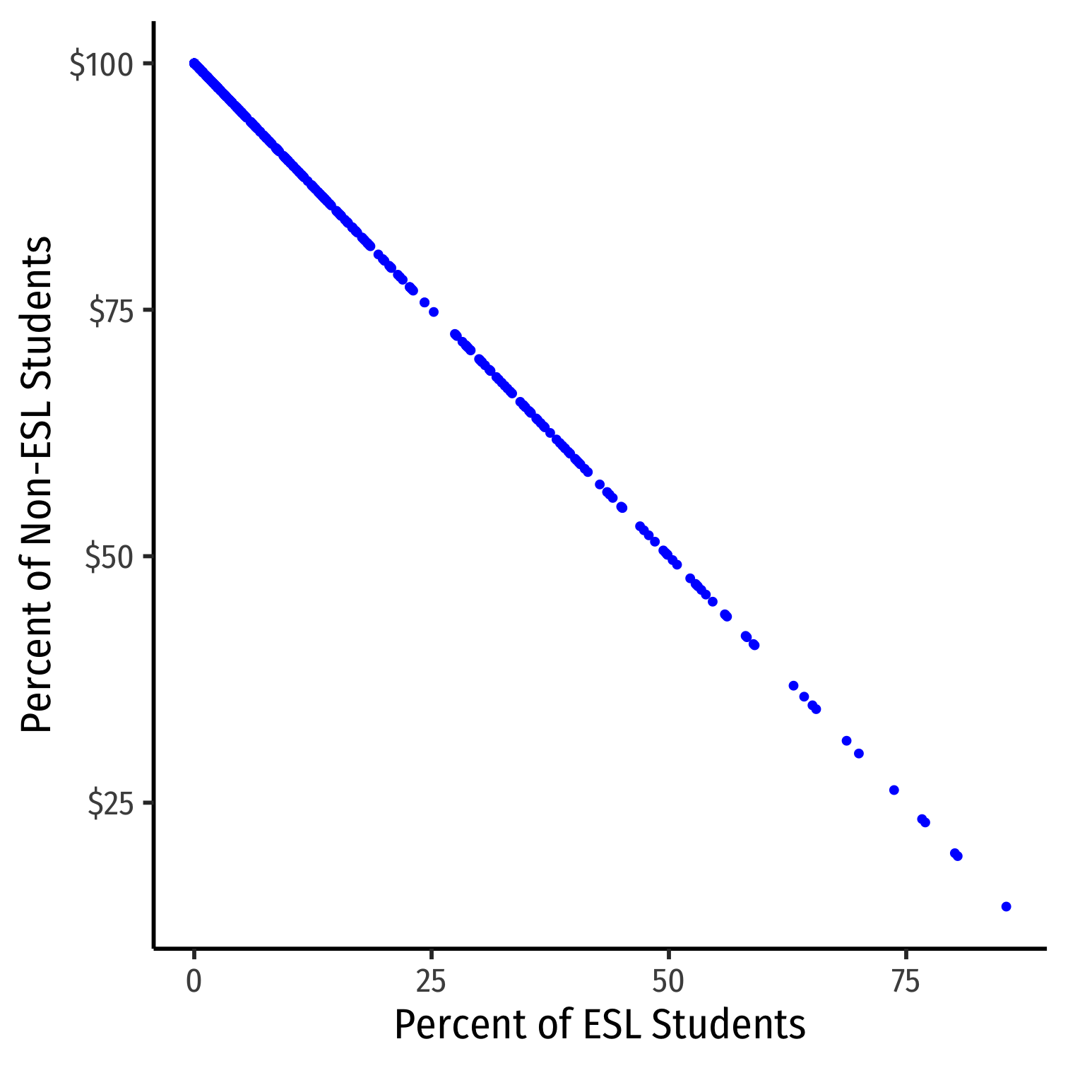
Perfect Multicollinearity Example IV
mcreg<-lm(testscr~str+el_pct+ef_pct, data=CASchool_ex)summary(mcreg)## ## Call:## lm(formula = testscr ~ str + el_pct + ef_pct, data = CASchool_ex)## ## Residuals:## Min 1Q Median 3Q Max ## -48.845 -10.240 -0.308 9.815 43.461 ## ## Coefficients: (1 not defined because of singularities)## Estimate Std. Error t value Pr(>|t|) ## (Intercept) 686.03225 7.41131 92.566 < 2e-16 ***## str -1.10130 0.38028 -2.896 0.00398 ** ## el_pct -0.64978 0.03934 -16.516 < 2e-16 ***## ef_pct NA NA NA NA ## ---## Signif. codes: 0 '***' 0.001 '**' 0.01 '*' 0.05 '.' 0.1 ' ' 1## ## Residual standard error: 14.46 on 417 degrees of freedom## Multiple R-squared: 0.4264, Adjusted R-squared: 0.4237 ## F-statistic: 155 on 2 and 417 DF, p-value: < 2.2e-16- Note
Rignores one of the multicollinear regressors (ef_pct) if you include both in a regression
A Summary of Multivariate OLS Estimator Properties
A Summary of Multivariate OLS Estimator Properties
^βj on Xj is biased only if there is an omitted variable (Z) such that:
- cor(Y,Z)≠0
- cor(Xj,Z)≠0
- If Z is included and Xj is collinear with Z, this does not cause a bias
var[^βj] and se[^βj] measure precision of estimate:
A Summary of Multivariate OLS Estimator Properties
^βj on Xj is biased only if there is an omitted variable (Z) such that:
- cor(Y,Z)≠0
- cor(Xj,Z)≠0
- If Z is included and Xj is collinear with Z, this does not cause a bias
var[^βj] and se[^βj] measure precision of estimate:
var[^βj]=1(1−R2j)∗SER2n×var[Xj]
- VIF from multicollinearity: 1(1−R2j)
- R2j for auxiliary regression of Xj on all other X's
- mutlicollinearity does not bias ^βj but raises its variance
- perfect multicollinearity if X's are linear function of others
Updated Measures of Fit
(Updated) Measures of Fit
Again, how well does a linear model fit the data?
How much variation in Yi is "explained" by variation in the model ($\hat{Y_i}$)?
(Updated) Measures of Fit
Again, how well does a linear model fit the data?
How much variation in Yi is "explained" by variation in the model ($\hat{Y_i}$)?
Yi=^Yi+^ui^ui=Yi−^Yi
(Updated) Measures of Fit: SER
- Again, the Standard errror of the regression (SER) estimates the standard error of u
SER=SSEn−k−1
A measure of the spread of the observations around the regression line (in units of Y), the average "size" of the residual
Only new change: divided by n−k−1 due to use of k+1 degrees of freedom to first estimate β0 and then all of the other β's for the k number of regressors1
1 Again, because your textbook defines (k) as including the constant, the denominator would be (n-k) instead of (n-k-1).
(Updated) Measures of Fit: R2
R2=ESSTSS=1−SSETSS=(rX,Y)2
- Again, R2 is fraction of variation of the model (^Yi ("explained SS") to the variation of observations of Yi ("total SS")
(Updated) Measures of Fit: Adjusted ˉR2
Problem: R2 of a regression increases every time a new variable is added (it reduces SSE!)
This does not mean adding a variable improves the fit of the model per se, R2 gets inflated
(Updated) Measures of Fit: Adjusted ˉR2
Problem: R2 of a regression increases every time a new variable is added (it reduces SSE!)
This does not mean adding a variable improves the fit of the model per se, R2 gets inflated
We correct for this effect with the adjusted R2:
ˉR2=1−n−1n−k−1×SSETSS
- There are different methods to compute ˉR2, and in the end, recall R2 was never very useful, so don't worry about knowing the formula
- Large sample sizes (n) make R2 and ˉR2 very close
In R (base)
## ## Call:## lm(formula = testscr ~ str + el_pct, data = CASchool)## ## Residuals:## Min 1Q Median 3Q Max ## -48.845 -10.240 -0.308 9.815 43.461 ## ## Coefficients:## Estimate Std. Error t value Pr(>|t|) ## (Intercept) 686.03225 7.41131 92.566 < 2e-16 ***## str -1.10130 0.38028 -2.896 0.00398 ** ## el_pct -0.64978 0.03934 -16.516 < 2e-16 ***## ---## Signif. codes: 0 '***' 0.001 '**' 0.01 '*' 0.05 '.' 0.1 ' ' 1## ## Residual standard error: 14.46 on 417 degrees of freedom## Multiple R-squared: 0.4264, Adjusted R-squared: 0.4237 ## F-statistic: 155 on 2 and 417 DF, p-value: < 2.2e-16- Base R2 (
Rcalls itmultiple R-squared) went up Adjusted R-squaredwent down
In R (broom)
elreg %>% glance()| r.squared | adj.r.squared | sigma | statistic | p.value | df | logLik | AIC | BIC | deviance | df.residual |
| 0.426 | 0.424 | 14.5 | 155 | 4.62e-51 | 3 | -1.72e+03 | 3.44e+03 | 3.46e+03 | 8.72e+04 | 417 |