Review: u

$$Y_i=\beta_0+\beta_1X_i+u_i$$

• Error term, \(u_i\) includes all other variables that affect \(Y\)

• Every regression model always has omitted variables assumed in the error

  • Most unobservable (hence "u") or hard to measure
  • Examples: innate ability, weather at the time, etc

• Again, we assume \(u\) is random, with \(E[u|X]=0\) and \(var(u)=\sigma^2_u\)

• Sometimes, omission of variables can bias OLS estimators \((\hat{\beta_0}\) and \(\hat{\beta_1})\)

Omitted Variable Bias I

• Omitted variable bias (OVB) for some omitted variable \(\mathbf{Z}\) exists if two conditionsa are met:

1. \(Z\) is a determinant of \(Y\)

• i.e. \(Z\) is in the error term, \(u_i\)

2. \(Z\) is correlated with the regressor \(X\)

• i.e. \(cor(X,Z) \neq 0\)

Omitted Variable Bias II

• Omitted variable bias makes \(X\) endogenous

  • \(E(\epsilon_i|X_i)\neq 0 \implies\) knowing \(X\) tells you something about \(\epsilon\)
    • Thus, \(X\) tells you something about \(Y\) not by way of \(X\)!

• \(\hat{\beta_1}\) is biased \(\left(E[\hat{\beta_1}] \neq \beta_1\right)\)

• Systematically over- or under-estimates the true relationship \((\beta_1)\)

• \(\hat{\beta_1}\) "picks up" both:

  • effect of \(X\rightarrow Y\)
  • effect of \(Z\rightarrow X \rightarrow X\)

Omited Variable Bias: Class Size Example

• Which of the following possible variables would cause a bias if omitted?

1. \(Z_i\): time of day of the test

2. \(Z_i\): parking space per student

3. \(Z_i\): percent of ESL students

Recall: Endogeneity and Bias

• The true expected value of \(\hat{\beta_1}\) is actually:¹

$$E[\hat{\beta_1}]=\beta_1+cor(X,u)\frac{\sigma_u}{\sigma_X}$$

• Takeaways:

1. If \(X\) is exogenous: \(cor(X,u)=0\), we're just left with \(\beta_1\)

2. The larger \(cor(X,u)\) is, larger bias: \(\left(E[\hat{\beta_1}]-\beta_1 \right)\)

3. We can "sign" the direction of the bias based on \(cor(X,u)\)

   • Positive \(cor(X,u)\) overestimates the true \(\beta_1\) \((\hat{\beta_1}\) is too high)
   • Negative \(cor(X,u)\) underestimates the true \(\beta_1\) \((\hat{\beta_1}\) is too low)

¹ See class class 2.4 notes for proof.

Endogeneity and Bias: Correlations I

• Here is where checking correlations between variables helps:

# Select only the three variables we want (there are many)
CAcorr<-CASchool %>%
  select("str","testscr","el_pct")
# Make a correlation table
corr<-cor(CAcorr)
corr

##                str    testscr     el_pct
## str      1.0000000 -0.2263628  0.1876424
## testscr -0.2263628  1.0000000 -0.6441237
## el_pct   0.1876424 -0.6441237  1.0000000

Endogeneity and Bias: Correlations II

• Here is where checking correlations between variables helps:

# Make a correlation plot
library(corrplot)
corrplot(corr, type="upper", 
         method = "number", # number for showing correlation coefficient
         order="original")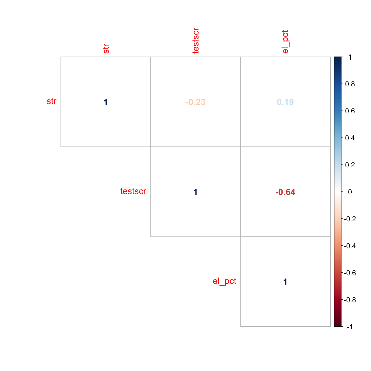

• el_pct is strongly correlated with testscr (Condition 1)
• el_pct is reasonably correlated with str (Condition 2)

Look at Conditional Distributions I

# make a new variable called EL
# = high (if el_pct is above median) or = low (if below median)
CASchool<-CASchool %>%
  mutate(ESL = ifelse(el_pct > median(el_pct),
                     "High ESL",
                     "Low ESL"))
# get average test score by high/low EL
CASchool %>%
  group_by(ESL) %>%
  summarize(Average_test_score=mean(testscr))

Look at Conditional Distributions II

ggplot(data = CASchool)+
  aes(x = testscr,
      fill = ESL)+
  geom_density(alpha=0.5)+
  labs(x = "Test Score",
       y = "Density")+
    theme_classic(base_family = "Fira Sans Condensed",
           base_size=20)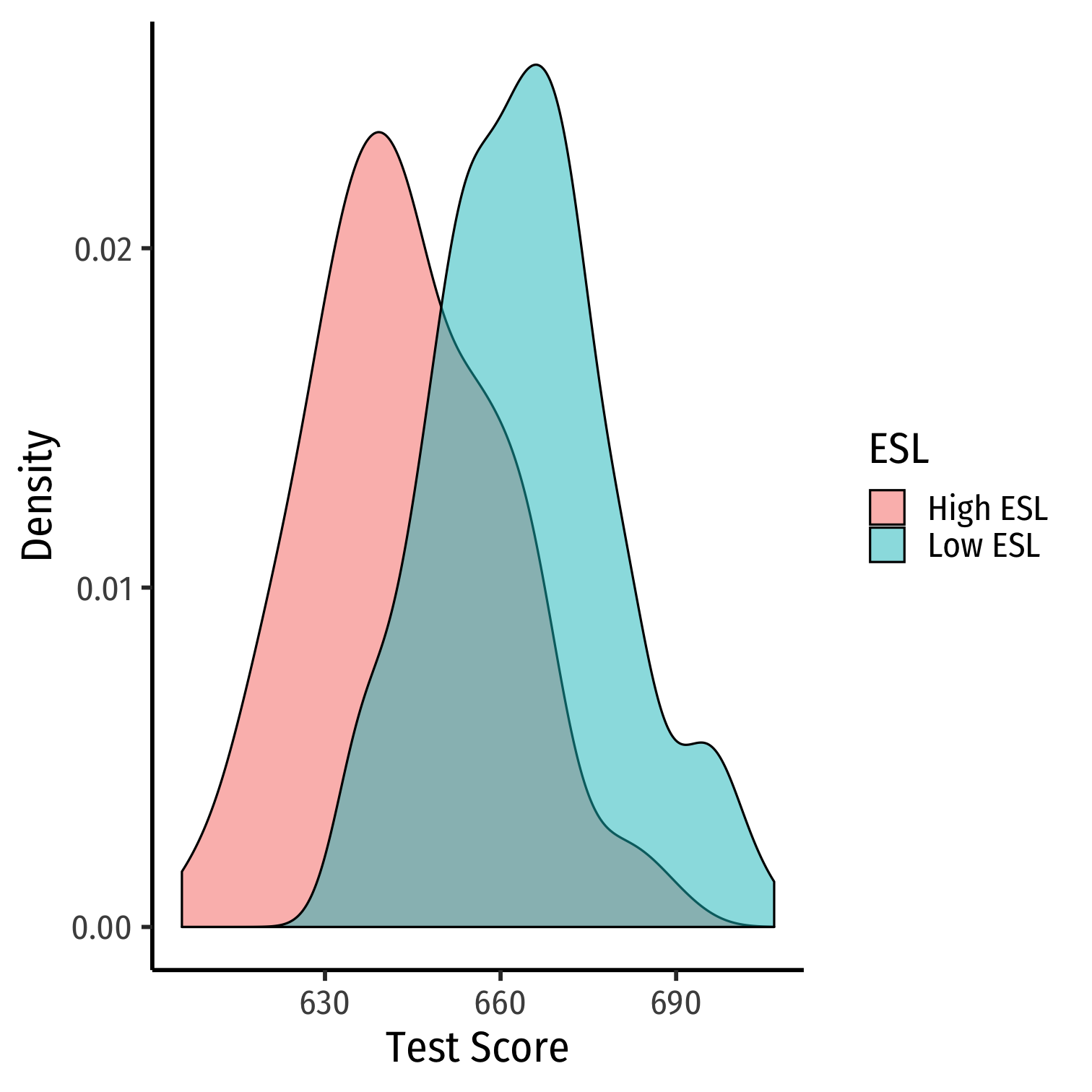

Look at Conditional Distributions III

cond_el_scatter<-ggplot(data = CASchool)+
  aes(x = str,
      y = testscr,
      color = ESL)+
  geom_point()+
  geom_smooth(method="lm")+
  labs(x = "STR",
       y = "Test Score")+
    theme_classic(base_family = "Fira Sans Condensed",
           base_size=20)
cond_el_scatter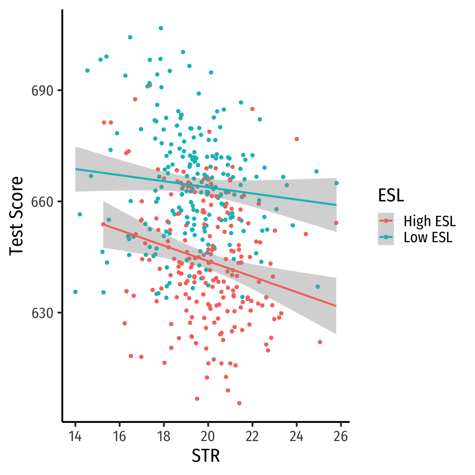

Look at Conditional Distributions III

cond_el_scatter+facet_grid(~ESL)+
  guides(color = F)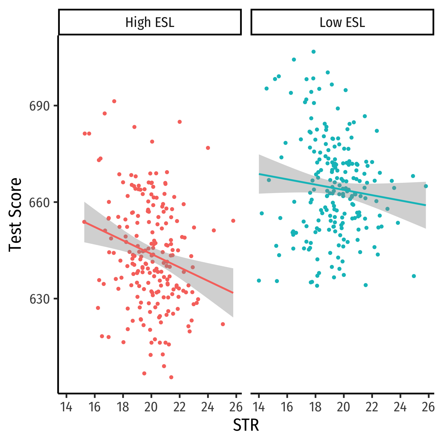

Omitted Variable Bias in the Class Size Example

$$E[\hat{\beta_1}]=\beta_1+bias$$ \(E[\hat{\beta_1}]=\) \(\beta_1\) \(+\) \(cor(X,u)\) \(\frac{\sigma_u}{\sigma_X}\)

• \(cor(STR,u)\) is positive (via \(\%EL\))

• \(cor(u, \text{Test score})\) is negative (via \(\%EL\))

• \(\beta_1\) is negative (between Test score and STR)

• Bias is positive

  • But since \\(\beta_1\\) is negative, it's made to be a more negative number than it truly is¹
  • Implies that \\(\beta_1\\) overstates the effect of reducing STR on improving Test Scores

¹ Hard to think about...but you'll see when we run the different regressions later!

Omitted Variable Bias: Messing with Causality I

If school districts with higher Test Scores happen to have both lower STR AND districts with smaller STR sizes tend to have less \(\%EL\) ...

• How can we say \(\hat{\beta_1}\) estimates the marginal effect of \(\Delta STR \rightarrow \Delta \text{Test Score}\)?

Omitted Variable Bias: Messing with Causality II

RCTs Neutralize Omitted Variable Bias I

RCTs Neutralize Omitted Variable Bias II

But We Rarely, if Ever, Have RCTs

There's Another Way to Reduce OVB

Multivariate Econometric Models Overview

$$Y_i = \beta_0 + \beta_1 X_{1i} + \beta_2 X_{2i} + \cdots + \beta_kX_{ki} +u_i$$

• \(Y\) is the dependent variable of interest
  • AKA "response variable," "regressand," "Left-hand side (LHS) variable"

• \(k\) number of independent variables \((X)\)'s
  • AKA "explanatory variables", "regressors," "Right-hand side (RHS) variables", "covariates"

• Our data consists of a spreadsheet of observed values of \((Y_i, X_{1i}, X_{2i}, \cdots ,X_{ki})\)

• To model, we "regress Y on \(X_1, X_2, \cdots, X_k\)"

• \(\beta_0, \beta_1, \cdots, \beta_k\) are parameters that describe the population relationships between the variables

  • We estimate \(k+1\) parameters ("betas")¹

¹ Note Bailey defines (k) to include both the number of variables plus the constant.

Marginal Effects I

$$Y_i= \beta_0+\beta_1 X_{1i} + \beta_2 X_{2i}$$

• Consider changing \(X_1\) by \(\Delta X_1\) while holding \(X_2\) constant:

$$\begin{align*} Y&= \beta_0+\beta_1 X_{1} + \beta_2 X_{2} && \text{Before the change}\\ \end{align*}$$

Marginal Effects I

$$Y_i= \beta_0+\beta_1 X_{1i} + \beta_2 X_{2i}$$

• Consider changing \(X_1\) by \(\Delta X_1\) while holding \(X_2\) constant:

$$\begin{align*} Y&= \beta_0+\beta_1 X_{1} + \beta_2 X_{2} && \text{Before the change}\\ Y+\Delta Y&= \beta_0+\beta_1 (X_{1}+\Delta X_1) + \beta_2 X_{2} && \text{After the change}\\ \end{align*}$$

Marginal Effects I

$$Y_i= \beta_0+\beta_1 X_{1i} + \beta_2 X_{2i}$$

• Consider changing \(X_1\) by \(\Delta X_1\) while holding \(X_2\) constant:

$$\begin{align*} Y&= \beta_0+\beta_1 X_{1} + \beta_2 X_{2} && \text{Before the change}\\ Y+\Delta Y&= \beta_0+\beta_1 (X_{1}+\Delta X_1) + \beta_2 X_{2} && \text{After the change}\\ \Delta Y&= \beta_1 \Delta X_1 && \text{The difference}\\ \end{align*}$$

Marginal Effects I

$$Y_i= \beta_0+\beta_1 X_{1i} + \beta_2 X_{2i}$$

• Consider changing \(X_1\) by \(\Delta X_1\) while holding \(X_2\) constant:

$$\begin{align*} Y&= \beta_0+\beta_1 X_{1} + \beta_2 X_{2} && \text{Before the change}\\ Y+\Delta Y&= \beta_0+\beta_1 (X_{1}+\Delta X_1) + \beta_2 X_{2} && \text{After the change}\\ \Delta Y&= \beta_1 \Delta X_1 && \text{The difference}\\ \frac{\Delta Y}{\Delta X_1} &= \beta_1 && \text{Solving for } \beta_1\\ \end{align*}$$

Marginal Effects II

$$\beta_1 =\frac{\Delta Y}{\Delta X_1}\text{ holding } X_2 \text{ constant}$$

Similarly, for \(\beta_2\):

$$\beta_2 =\frac{\Delta Y}{\Delta X_2}\text{ holding }X_1 \text{ constant}$$

And for the constant, \(\beta_0\):

$$\beta_0 =\text{predicted value of Y when } X_1=0, \; X_2=0$$

You Can Keep Your Intuitions...But They're Wrong Now

The "Constant"

• Alternatively, we can write the population regression equation as: $$Y_i=\beta_0\mathbf{X_{0i}}+\beta_1X_{1i}+\beta_2X_{2i}+u_i$$

• Here, we added \(X_{0i}\) to \(\beta_0\)

• \(X_{0i}\) is a constant regressor, as we define \(X_{0i}=1\) for all \(i\) observations

• Likewise, \(\beta_0\) is more generally called the constant term in the regression (instead of the "intercept")

• This may seem silly and trivial, but this will be important soon!

The Population Regression Model: Example I

• Let's see what you remember from micro(econ)!

• What measures the price effect? What sign should it have?

• What measures the income effect? What sign should it have? What should inferior or normal (necessities & luxury) goods look like?

• What measures the cross-price effect(s)? What sign should substitutes and complements have?

The Population Regression Model: Example I

• Interpret each \(\hat{\beta}\)

Multivariate OLS in R

# run regression of testscr on str and el_pct
school_reg_2 <- lm(testscr ~ str+el_pct, 
                 data = CASchool)

Multivariate OLS in R II

# look at reg object
school_reg_2

## 
## Call:
## lm(formula = testscr ~ str + el_pct, data = CASchool)
## 
## Coefficients:
## (Intercept)          str       el_pct  
##    686.0322      -1.1013      -0.6498

Multivariate OLS in R III

summary(school_reg_2) # get full summary

## 
## Call:
## lm(formula = testscr ~ str + el_pct, data = CASchool)
## 
## Residuals:
##     Min      1Q  Median      3Q     Max 
## -48.845 -10.240  -0.308   9.815  43.461 
## 
## Coefficients:
##              Estimate Std. Error t value Pr(>|t|)    
## (Intercept) 686.03225    7.41131  92.566  < 2e-16 ***
## str          -1.10130    0.38028  -2.896  0.00398 ** 
## el_pct       -0.64978    0.03934 -16.516  < 2e-16 ***
## ---
## Signif. codes:  0 '***' 0.001 '**' 0.01 '*' 0.05 '.' 0.1 ' ' 1
## 
## Residual standard error: 14.46 on 417 degrees of freedom
## Multiple R-squared:  0.4264,    Adjusted R-squared:  0.4237 
## F-statistic:   155 on 2 and 417 DF,  p-value: < 2.2e-16

Multivariate OLS in R IV: broom

# load packages
library(broom)
# tidy regression output
tidy(school_reg_2)

Multivariate Regression Output Table

library(huxtable)
huxreg("Model 1" = school_reg,
       "Model 2" = school_reg_2,
       coefs = c("Intercept" = "(Intercept)",
                 "Class Size" = "str",
                 "%ESL Students" = "el_pct"),
       statistics = c("N" = "nobs",
                      "R-Squared" = "r.squared",
                      "SER" = "sigma"),
       number_format = 2)