The Sampling Distribution of ^β1
^β1∼N(E[^β1],σ^β1)
E[^β1]; the center of the distribution (2 classes ago)
- E[^β1]=β11
σ^β1; how precise is our estimate? (last class)
- Variance σ2^β1 or standard error σ^β1
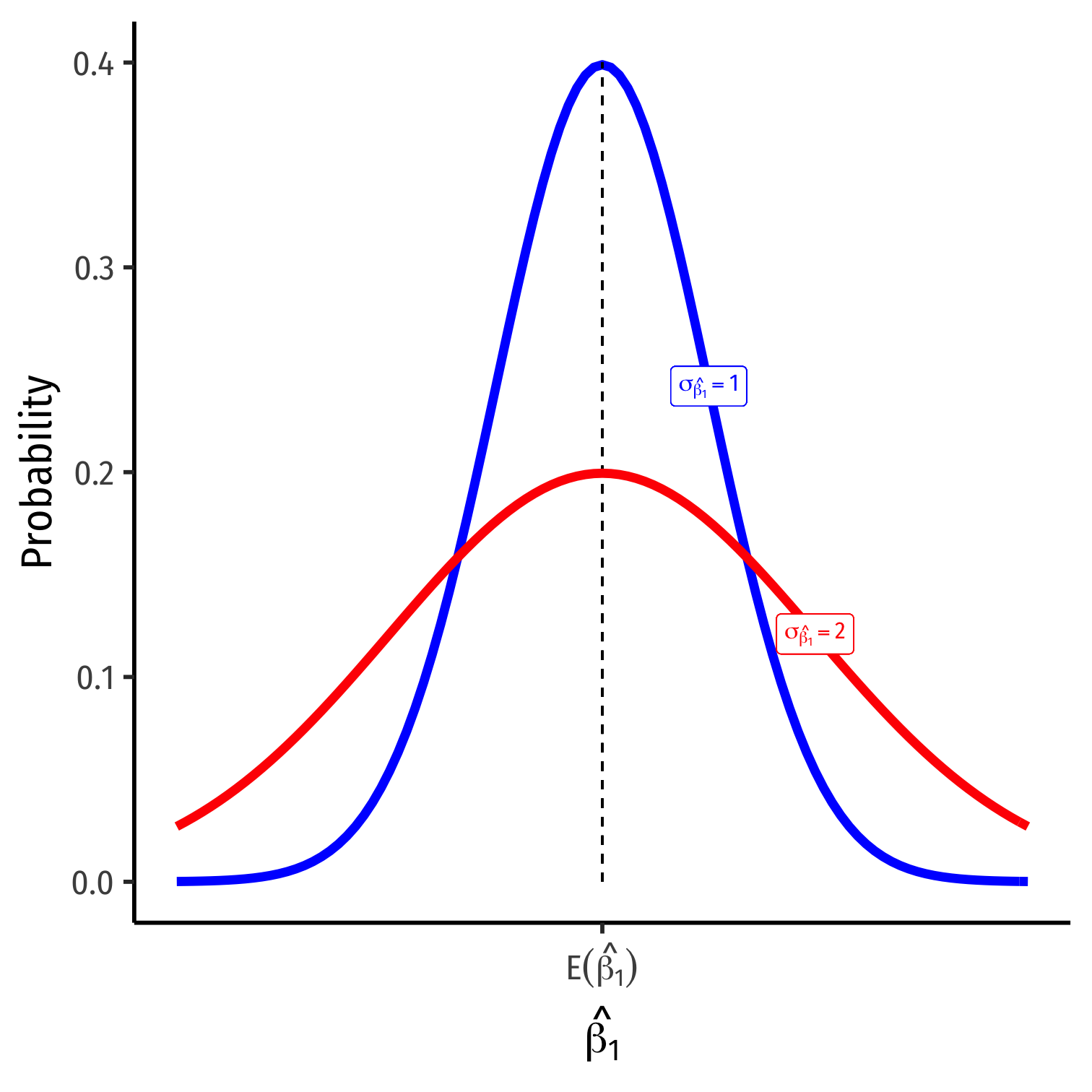
1 Under the 4 assumptions about u (particularly, cor(X,u)=0).
Recall: The Two Big Problems with Data
- We use econometrics to identify causal relationships and make inferences about them
Problem for identification: endogeneity
- X is exogenous if its variation is unrelated to other factors (u) that affect Y
- X is endogenous if its variation is related to other factors (u) that affect Y
Problem for inference: randomness
- Data is random due to natural sampling variation
- Taking one sample of a population will yield slightly different information than another sample of the same population


Recall: Inferential Statistics and Sampling Distributions
Inferential statistics analyzes a sample to make inferences about a much larger (unobservable) population
Population: all possible individuals that match some well-defined criterion of interest (people, firms, cities, etc)
- Characteristics about (relationships between variables in) populations are called parameters
Sample: some portion of the population of interest to represent the whole
- Samples generate statistics used to estimate population parameters

Type I and Type II Errors I
Any sample statistic (e.g. ^β1) will rarely be exactly equal to the hypothesized population parameter (e.g. β1)
Difference between observed statistic and true paremeter could be because:
Parameter is not the hypothesized value (H0 is false)
Parameter is truly the hypothesized value (H0 is true) but sampling variability gave us a different estimate
- We cannot distinguish between these two possibilities with any certainty

Type I and Type II Errors II
- We can interpret our estimates probabilistically as commiting one of two types of error:
Type I error (false positive): rejecting H0 when it is in fact true
- Believing we found an important result when there is truly no relationship
Type II error (false negative): failing to reject H0 when it is in fact false
- Believing we found nothing when there was truly a relationship to find
Type I and Type II Errors V

William Blackstone
(1723-1780)
"It is better that ten guilty persons escape than that one innocent suffer."
- Type I error is worse than a Type II error in law!
Blackstone, William, 1765-1770, Commentaries on the Laws of England
Type I and Type II Errors VI

Hypothesis Testing and the Philosophy of Science I

Sir Ronald A. Fisher
(1890—1962)
"The null hypothesis is never proved or established, but is possibly disproved, in the course of experimentation. Every experiment may be said to exist only in order to give the facts a chance of disproving the null hypothesis."
1931, The Design of Experiments
Hypothesis Testing and the Philosophy of Science I
Modern philosophy of science is largely based off of hypothesis testing and falsifiability, which form the "Scientific Method"1
For something to be "scientific", it must be falsifiable, or at least testable
Hypotheses can be corroborated with evidence, but always tentative until falsified by data in suggesting an alternative hypothesis
"All swans are white" is a hypothesis rejected upon discovery of a single black swan

Hypothesis Testing: Which Test? II

Elements of a Hypothesis Test

Hypothesis Testing with the infer Package II

Hypothesis Testing with the infer Package II

Hypothesis Testing with the infer Package II

Hypothesis Testing with the infer Package II

Hypothesis Testing with the infer Package II

Hypothesis Testing with the infer Package II

Imagine a Null World, where H0 is True

Our world, and a world where β1=0 by assumption.
The infer Pipeline: Specify
The infer Pipeline: Hypothesize
The infer Pipeline: Generate I
The infer Pipeline: Calculate I
The infer Pipeline: Visualize I
The infer Pipeline: Visualize I
Specify
Hypothesize
Generate
Calculate
Visualize
%>% visualize()- Make a histogram of our null distribution of β1
- Note it is centered at β1=0 because that's H0!
simulations %>% visualize()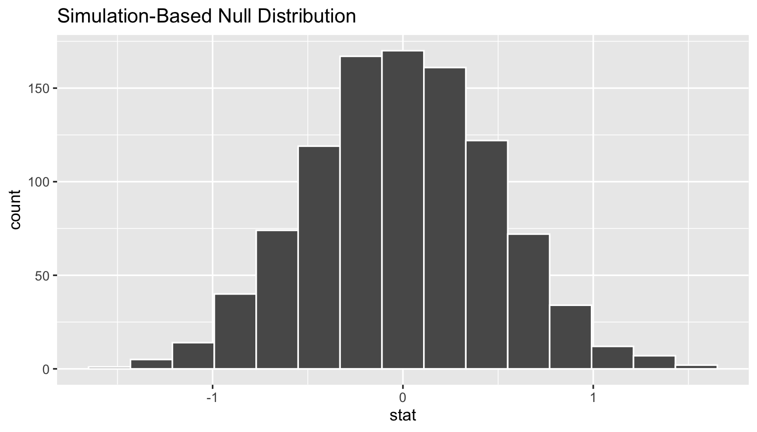
The infer Pipeline: Visualize II
Specify
Hypothesize
Generate
Calculate
Visualize
%>% visualize()- Add our
sample_slopeto show our finding on the null distr.
simulations %>% visualize(obs_stat = sample_slope)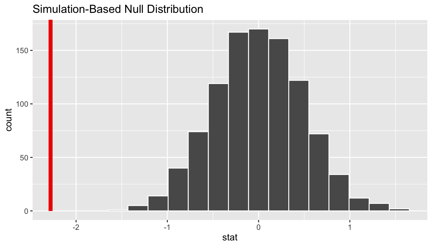
The infer Pipeline: Visualize p-value
Specify
Hypothesize
Generate
Calculate
Visualize
%>% visualize()+ shade_p_value()- Add
shade_p_valueto see what p is
simulations %>% visualize(obs_stat = sample_slope)+ shade_p_value(obs_stat = sample_slope, direction = "two_sided")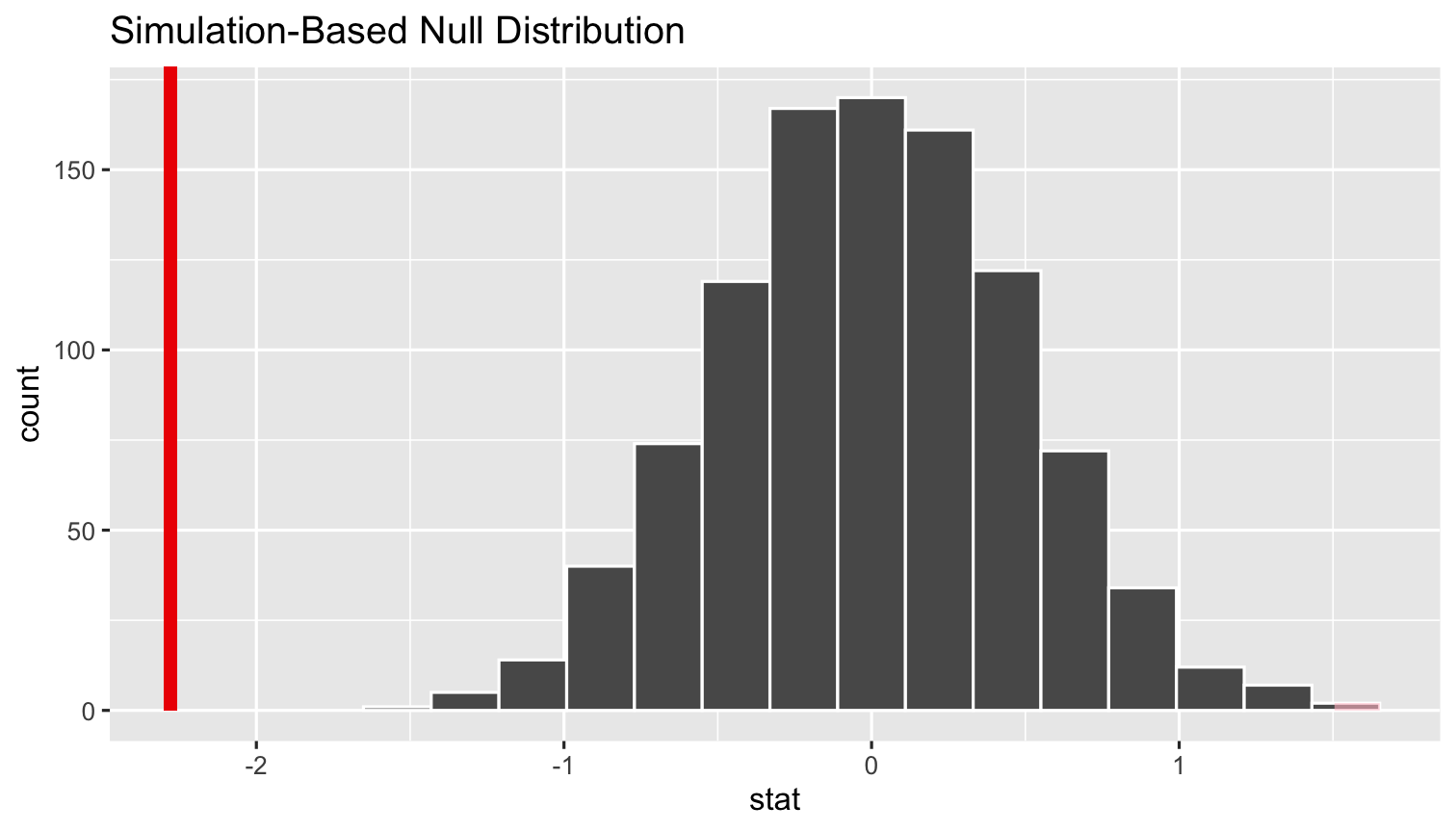
The infer Pipeline: Visualize Confidence Intervals
Specify
Hypothesize
Generate
Calculate
Visualize
%>% visualize()+ shade_ci()- To shade confidence interval, we first need a vector of what they are
- I've saved the outputted
tibbleof them from 4 slides ago asci_values
- I've saved the outputted
simulations %>% visualize(obs_stat = sample_slope)+ shade_confidence_interval(ci_values)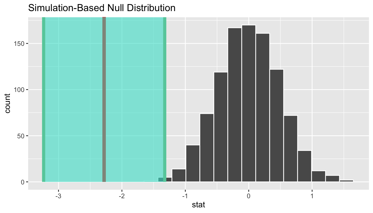
The infer Pipeline: Visualize is a Wrapper of ggplot
infer'svisualize()function is just a wrapper function forggplot()- you can take your
simulationstibbleand justggplota normal histogram
- you can take your
simulations %>% ggplot(data = .)+ aes(x = stat)+ geom_histogram(color="white", fill="indianred")+ geom_vline(xintercept = sample_slope, color = "blue", size = 2, linetype = "dashed")+ labs(x = expression(paste("Distribution of ", hat(beta[1]), " under ", H[0], " that ", beta[1]==0)), y = "Samples")+ theme_classic(base_family = "Fira Sans Condensed", base_size=20)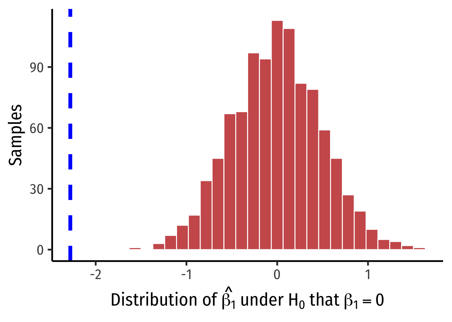
What R Does: Classical Statistical Inference I
R does things the old-fashioned way, using a theoretical null distribution instead of simulation
A t-distribution with n−k−1 df1
Calculate a t-statistic for ^β1:
test statistic=estimate−null hypothesisstandard error of estimate
1 k is the number of X variables.
What R Does: Classical Statistical Inference II
test statistic=estimate−null hypothesisstandard error of estimate
t has the same interpretation as Z, number of std. dev. away from the distribution's center1
Compares to a critical value of t∗ (determined by α & n−k−1)
- For 95% confidence, α=0.05, t∗≈22

1 Think of our simulated distribution, the center was 0.
2 The 68-95-99.7% empirical rule!
What R Does: Classical Statistical Inference III
t=^β1−β1,0se(^β1)t=−2.28−00.48t=−4.75
Our sample slope is 4.75 standard deviations below the mean under H0
p-value: prob. of a test statistic at least as large (in magnitude) as ours if the null hypothesis were true1
- p-value is 2-sided for Ha:β1≠0

1 Think of our simulated distribution, the center was 0.
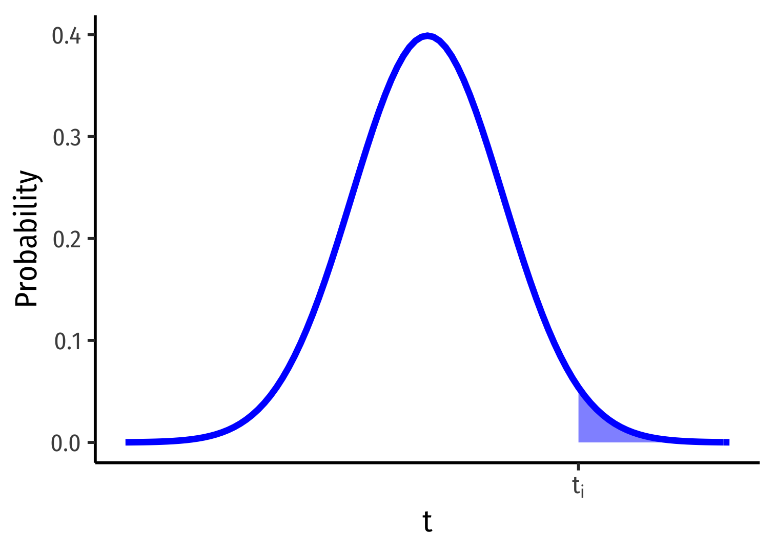
1-Sided vs. 2-Sided p-values I
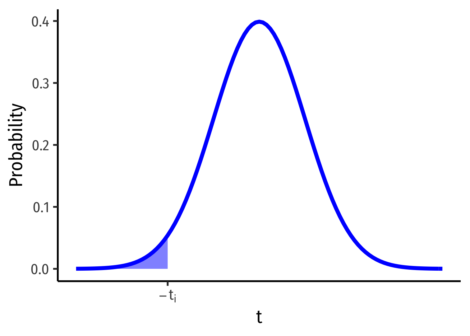
Ha:β1<0
p-value: Prob(t<ti)
Ha:β1>0
p-value: Prob(t>ti)
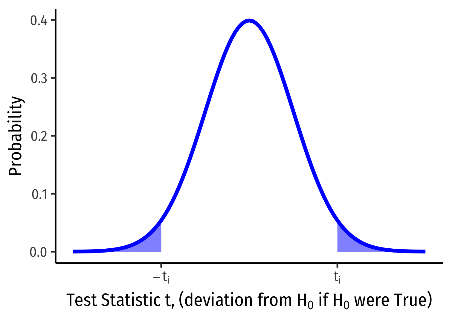
1-Sided vs. 2-Sided p-values I
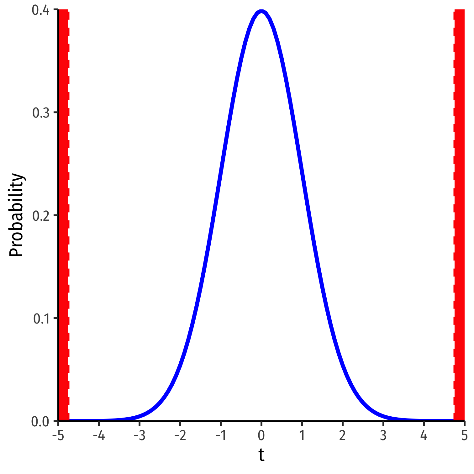
Ha:β1≠0
p-value: 2×Prob(t>|ti|)
Abusing p-Values I


Abusing p-Values II

"The widespread use of 'statistical significance' (generally interpreted as (p≤0.05) as a license for making a claim of a scientific finding (or implied truth) leads to considerable distortion of the scientific process."
Wasserstein, Ronald L. and Nicole A. Lazar, (2016), "The ASA's Statement on p-Values: Context, Process, and Purpose," The American Statistician 30(2): 129-133