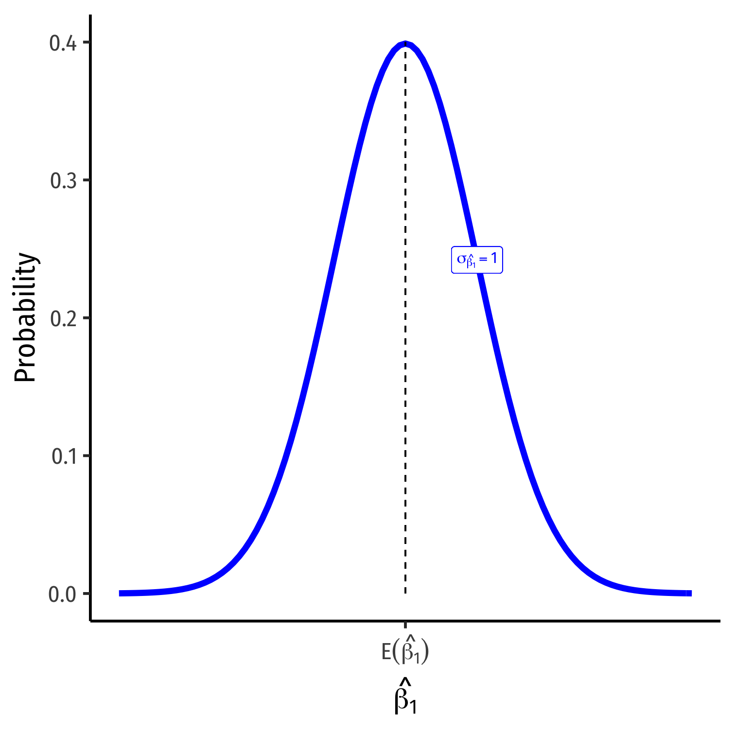
The Sampling Distribution of \(\hat{\beta_1}\)
$$\hat{\beta_1} \sim N(E[\hat{\beta_1}], \sigma_{\hat{\beta_1}})$$
- \(E[\hat{\beta_1}]\); the center of the distribution (last class)
- \(E[\hat{\beta_1}]=\beta_1\)1
The Sampling Distribution of \(\hat{\beta_1}\)
$$\hat{\beta_1} \sim N(E[\hat{\beta_1}], \sigma_{\hat{\beta_1}})$$
\(E[\hat{\beta_1}]\); the center of the distribution (last class)
- \(E[\hat{\beta_1}]=\beta_1\)1
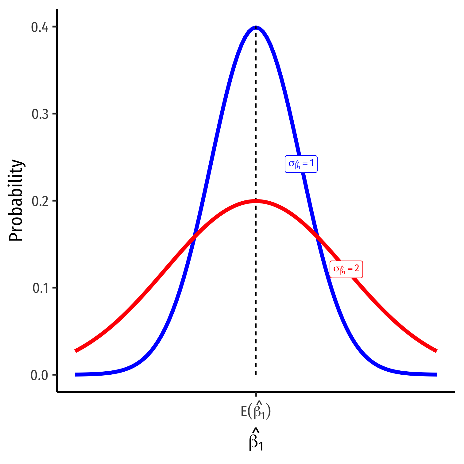
\(\sigma_{\hat{\beta_1}}\); how precise is our estimate? (today)
- Variance \(\sigma^2_{\hat{\beta_1}}\) or standard error+ \(\sigma_{\hat{\beta_1}}\)
1 Under the 4 assumptions about \(u\) (particularly, \(cor(X,u)=0)\).
+ Standard "error" is the analog of standard deviation when talking about
the sampling distribution of a sample statistic (such as \(\bar{X}\) or \(\hat{\beta_1})\).
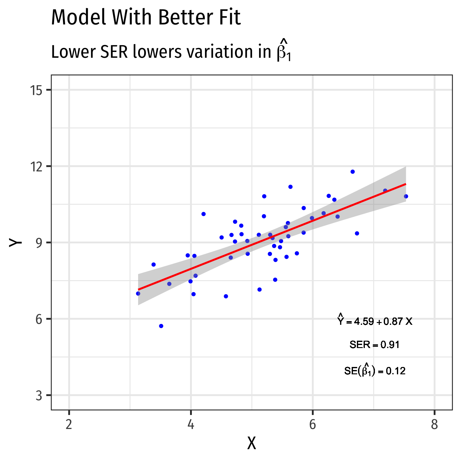
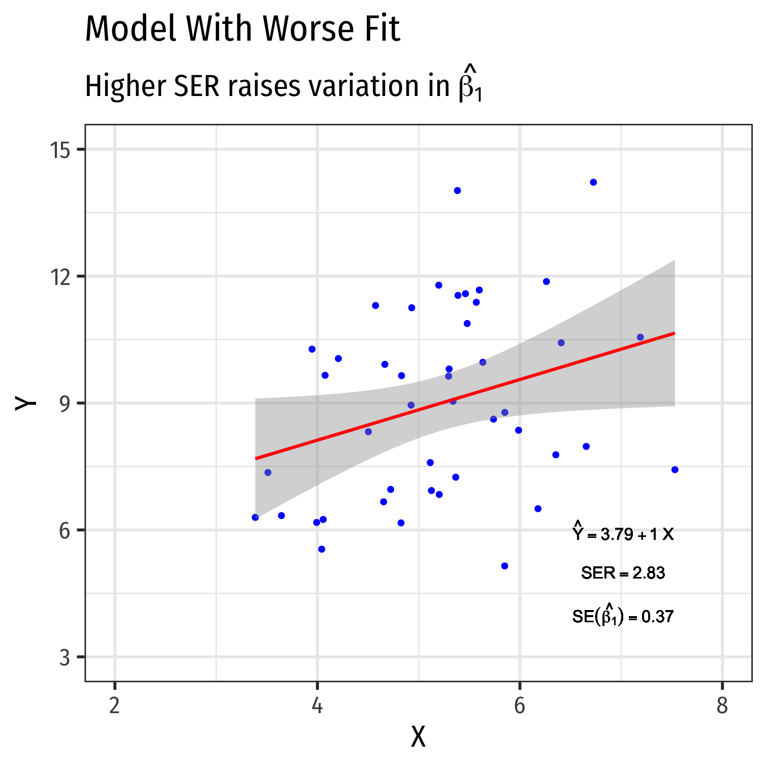
Variation in \(\hat{\beta_1}\): Goodness of Fit
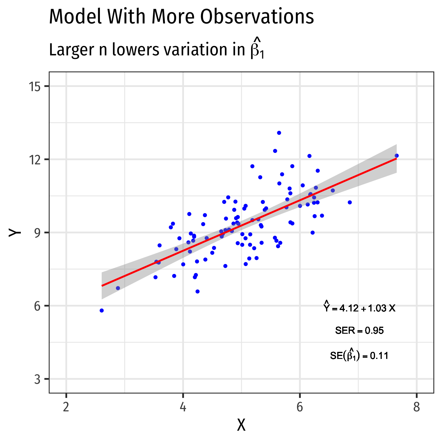
Variation in \(\hat{\beta_1}\): Sample Size

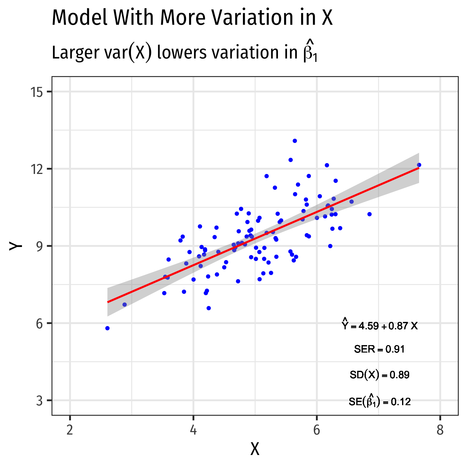
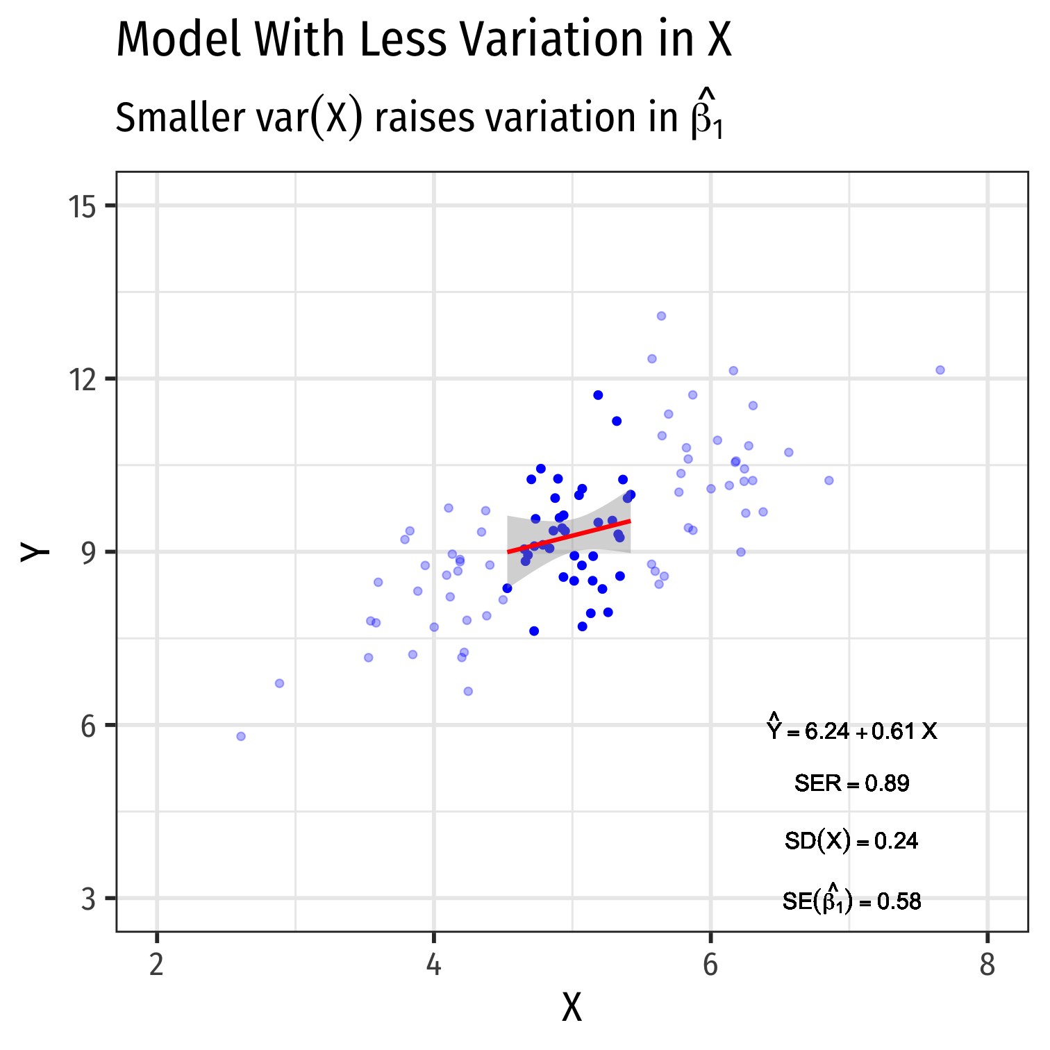
Variation in \(\hat{\beta_1}\): Variation in \(X\)
Recap: Assumptions about Errors
- Recall the 4 critical assumptions about \(u\):
The expected value of the residuals is 0 $$E[u]=0$$
The variance of the residuals over \(X\) is constant, written: $$var(u|X)=\sigma^2_{u}$$
Errors are not correlated across observations: $$cor(u_i,u_j)=0 \quad \forall i \neq j$$
No correlation between \(X\) and the error term: $$cor(X, u)=0 \text{ or } E[u|X]=0$$

Plotting Residuals
ggplot(data = aug_reg)+ aes(x = .resid)+ geom_histogram(color="white")+ labs(x = expression(paste("Residual, ", hat(u))))+ theme_bw(base_family = "Fira Sans Condensed", base_size=20)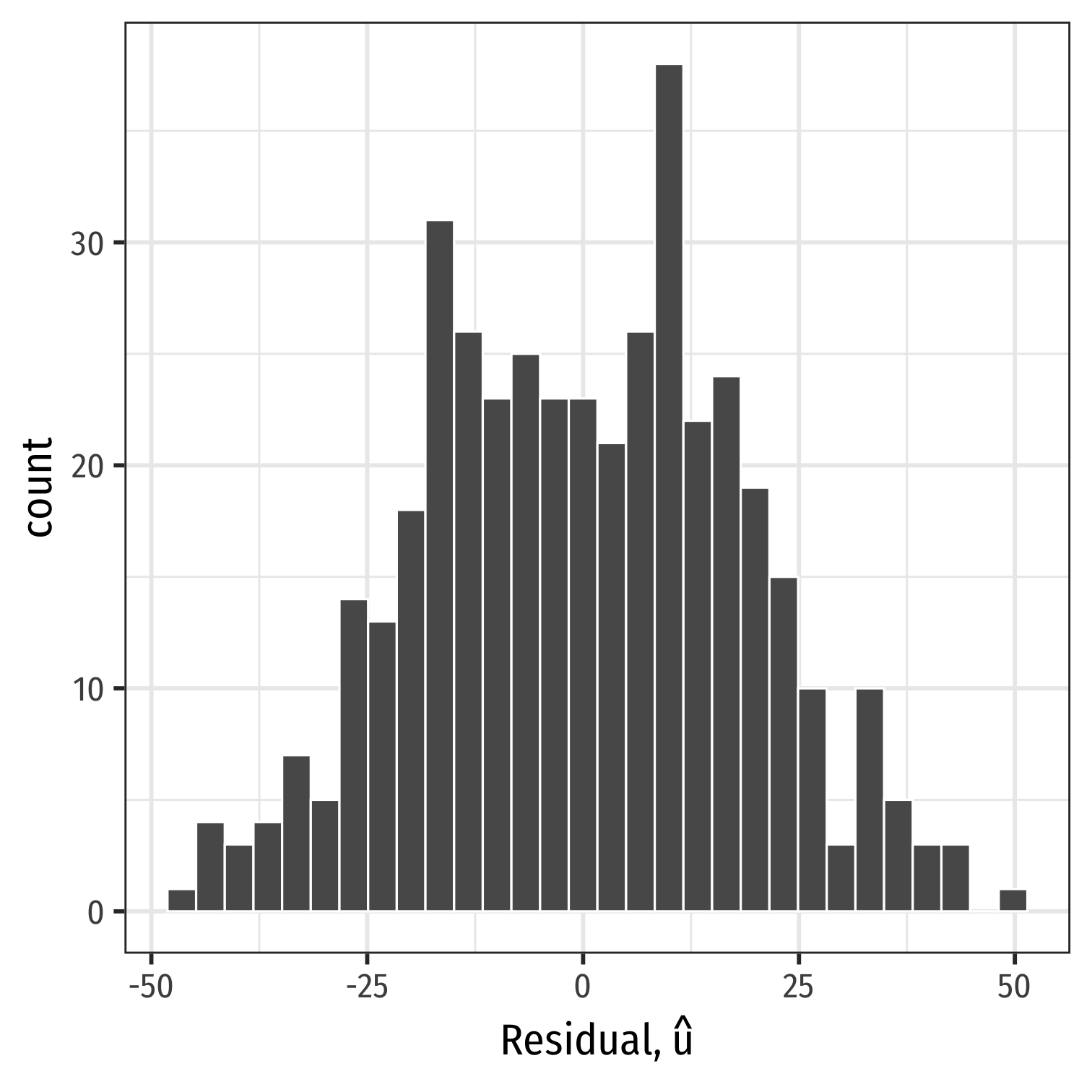
Plotting Residuals
ggplot(data = aug_reg)+ aes(x = .resid)+ geom_histogram(color="white")+ labs(x = expression(paste("Residual, ", hat(u))))+ theme_bw(base_family = "Fira Sans Condensed", base_size=20)- Just to check:
aug_reg %>% summarize(E_u = mean(.resid), sd_u = sd(.resid))| E_u | sd_u |
| -5.76e-16 | 18.6 |

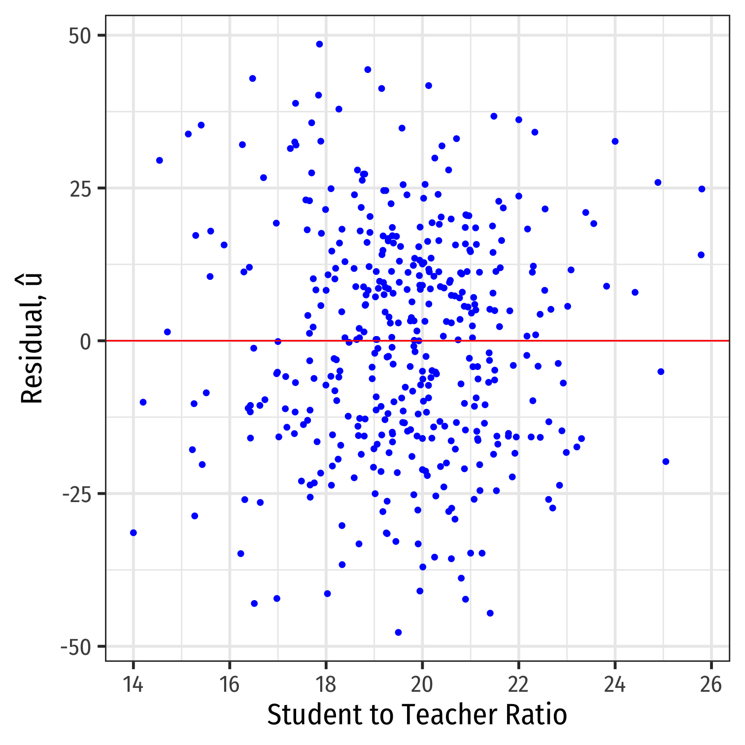
Residual Plot
- We often plot a residual plot to see any odd patterns about residuals
- \(x\)-axis are \(X\) values (
str) - \(y\)-axis are \(u\) values (
.resid)
- \(x\)-axis are \(X\) values (
Homoskedasticity
"Homoskedasticity:" variance of the residuals over \(X\) is constant, written: $$var(u|X)=\sigma^2_{u}$$
Knowing the value of \(X\) does not affect the variance (spread) of the errors
Heteroskedasticity I
"Heteroskedasticity:" variance of the residuals over \(X\) is NOT constant: $$var(u|X) \neq \sigma^2_{u}$$
This does not cause \(\hat{\beta_1}\) to be biased, but it does cause the standard error of \(\hat{\beta_1}\) to be incorrect
This does cause a problem for inference!
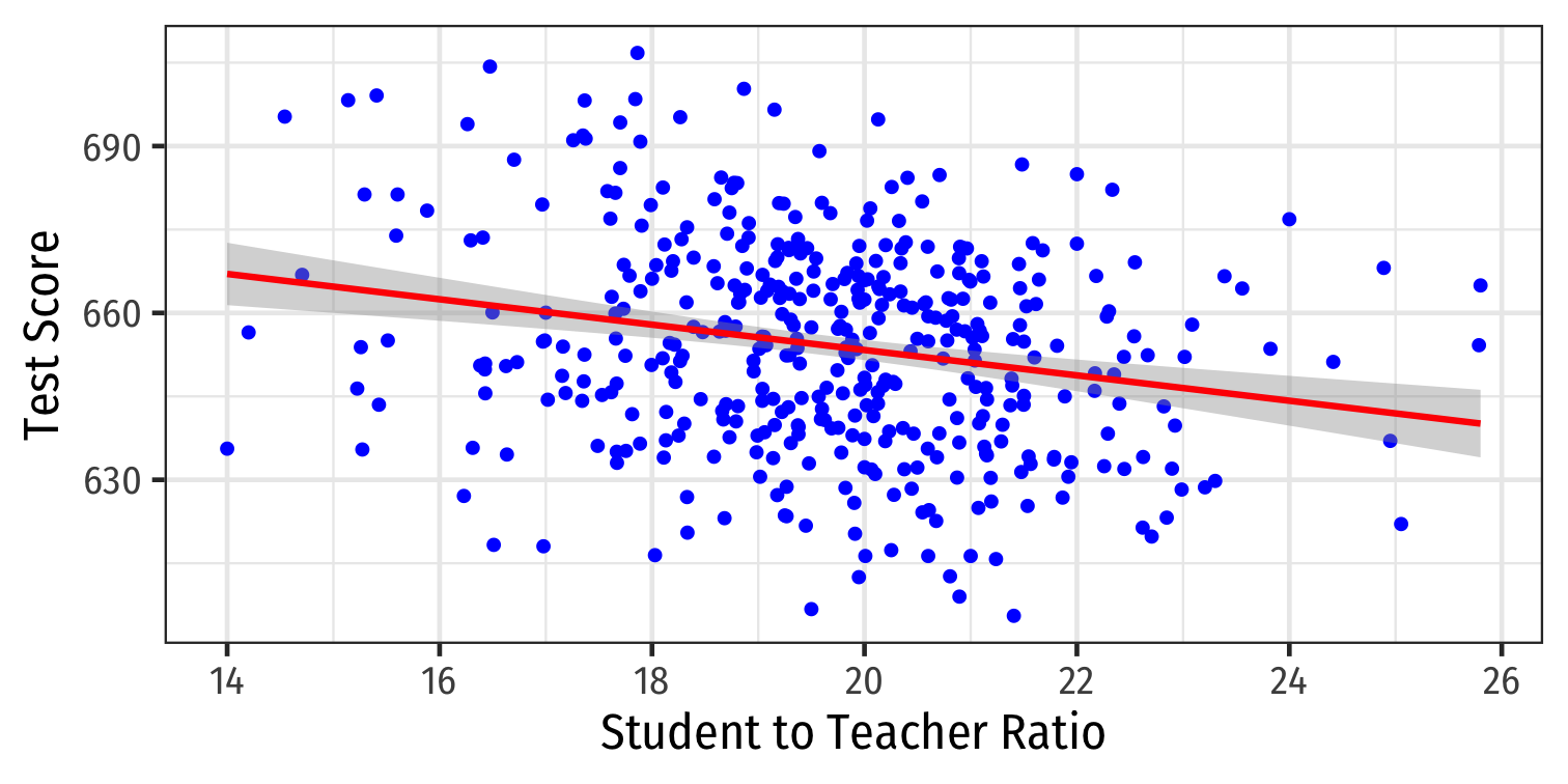
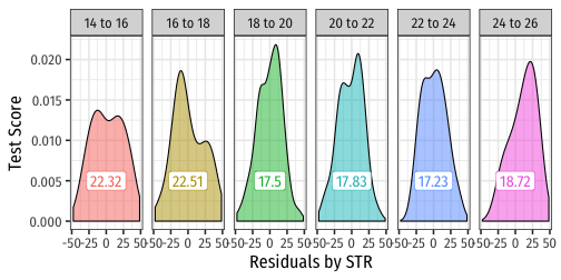
Visualizing Heteroskedasticity I
- Our original scatterplot with regression line
Visualizing Heteroskedasticity I
Our original scatterplot with regression line
Does the spread of the errors change over different values of \(str\)?
- No: homoskedastic
- Yes: heteroskedastic

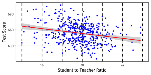
Visualizing Heteroskedasticity I
Our original scatterplot with regression line
Does the spread of the errors change over different values of \(str\)?
- No: homoskedastic
- Yes: heteroskedastic
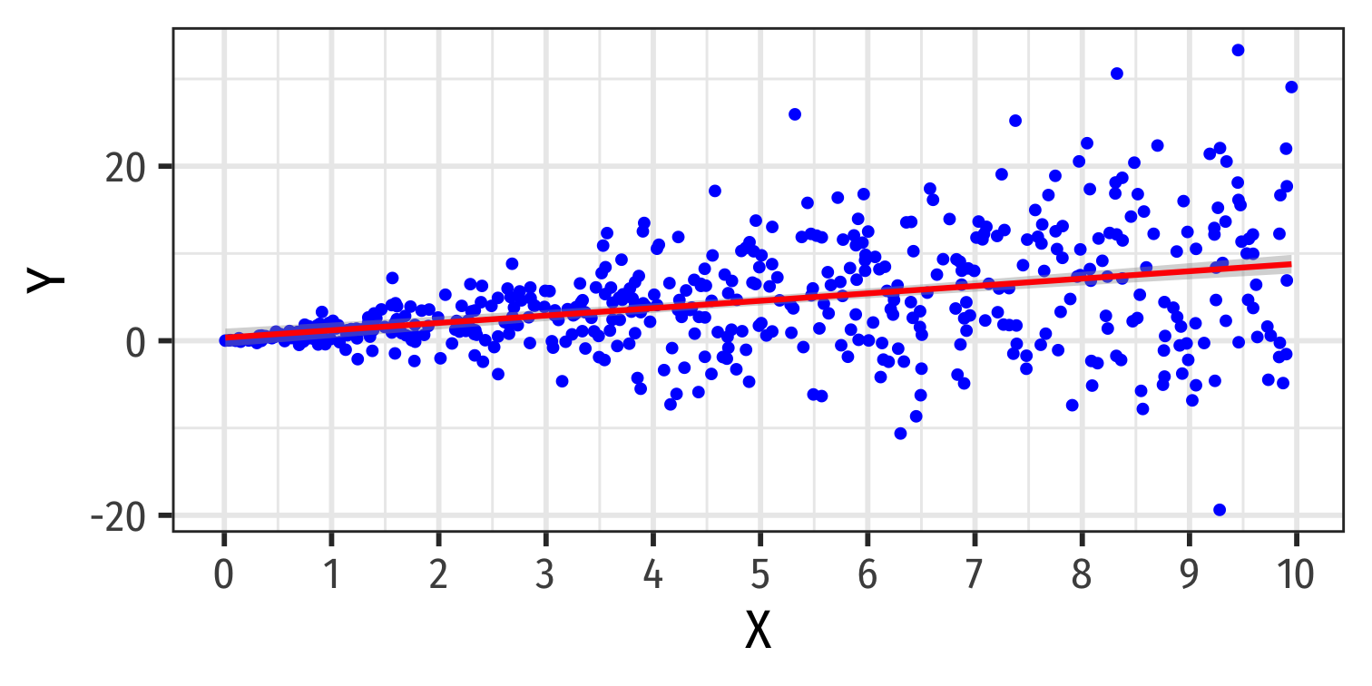
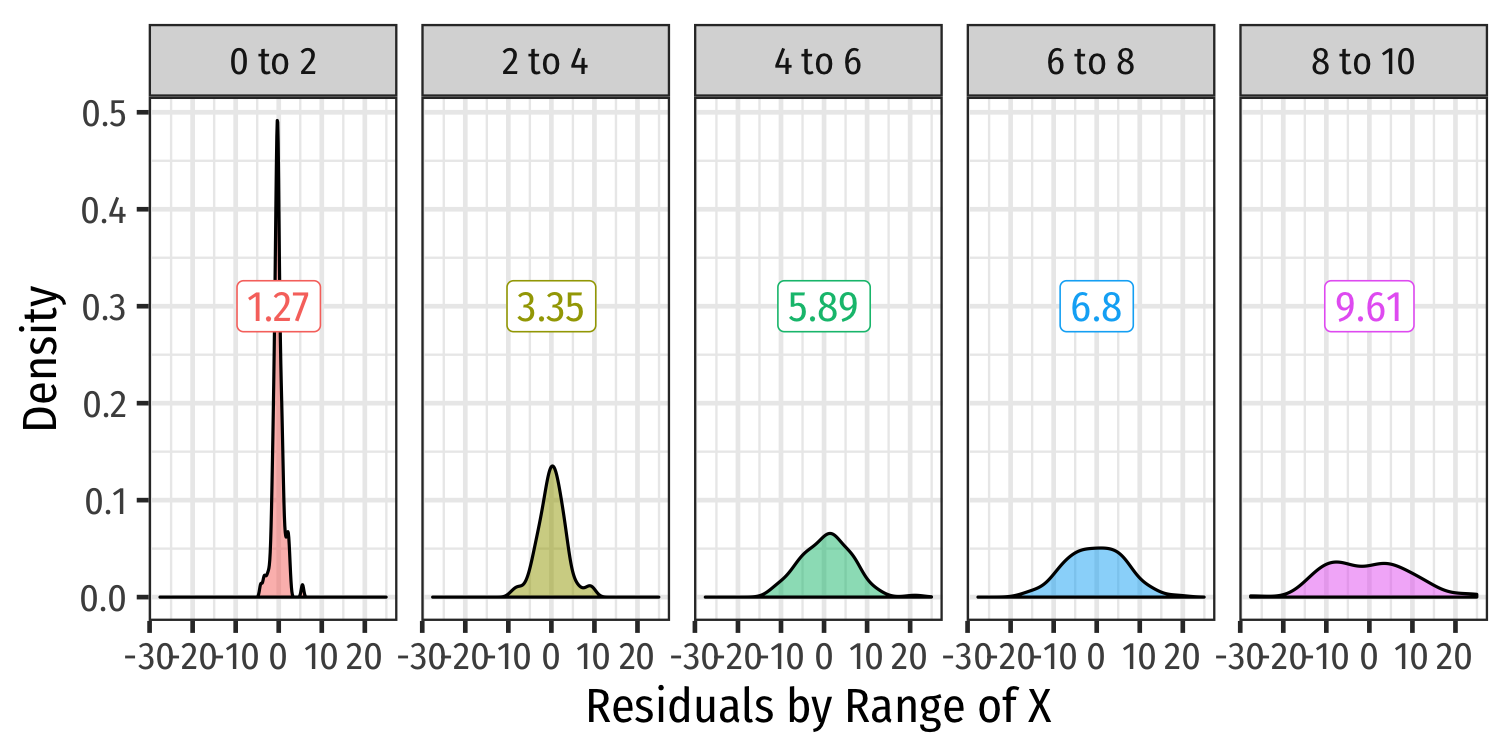
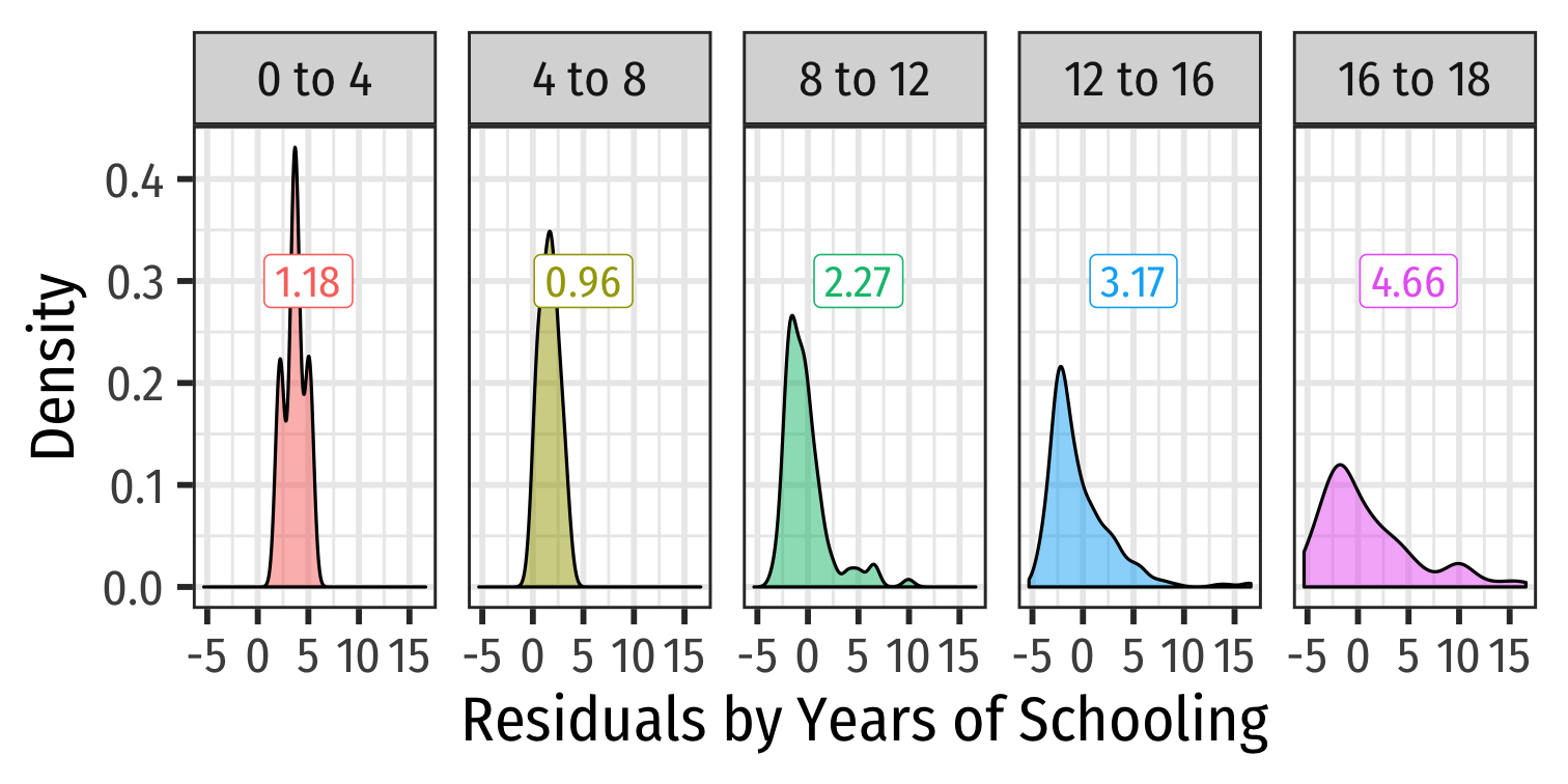
More Obvious Heteroskedasticity
- Visual cue: data is "fan-shaped"
- Data points are closer to line in some areas
- Data points are more spread from line in other areas
More Obvious Heteroskedasticity
- Visual cue: data is "fan-shaped"
- Data points are closer to line in some areas
- Data points are more spread from line in other areas

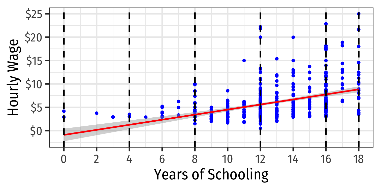
What Might Cause Heteroskedastic Errors?
$$\widehat{wage_i}=\hat{\beta_0}+\hat{\beta_1}educ_i$$
| Wage | |
| Intercept | -0.90 |
| (0.68) | |
| Years of Schooling | 0.54 *** |
| (0.05) | |
| N | 526 |
| R-Squared | 0.16 |
| SER | 3.38 |
| *** p < 0.001; ** p < 0.01; * p < 0.05. | |
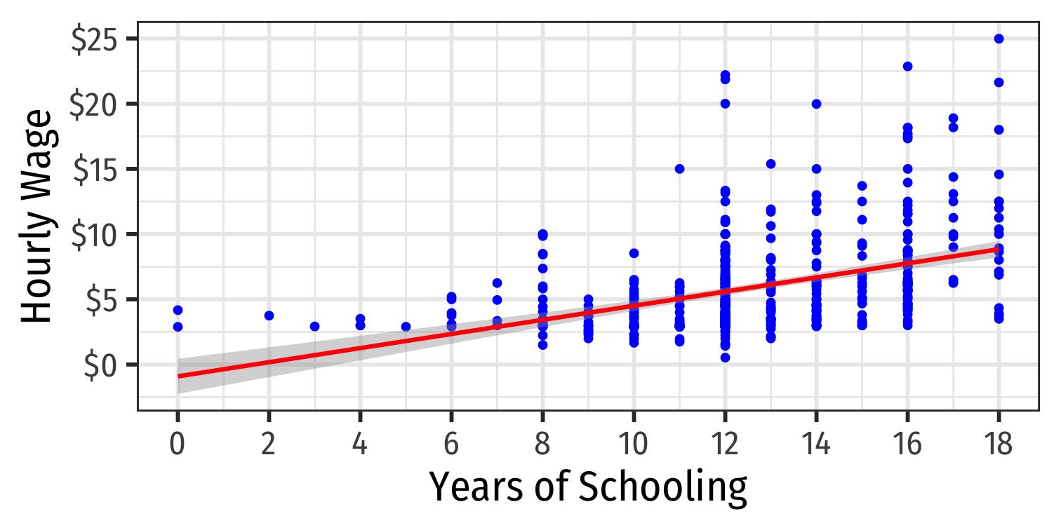
What Might Cause Heteroskedastic Errors?
$$\widehat{wage_i}=\hat{\beta_0}+\hat{\beta_1}educ_i$$
| Wage | |
| Intercept | -0.90 |
| (0.68) | |
| Years of Schooling | 0.54 *** |
| (0.05) | |
| N | 526 |
| R-Squared | 0.16 |
| SER | 3.38 |
| *** p < 0.001; ** p < 0.01; * p < 0.05. | |
Assumption 3: No Serial Correlation
Errors are not correlated across observations: $$cor(u_i,u_j)=0 \quad \forall i \neq j$$
For simple cross-sectional data, this is rarely an issue
Time-series & panel data nearly always contain serial correlation or autocorrelation between errors
Errors may be clustered
- by group: e.g. all observations from Maryland, all observations from Virginia, etc.
- by time: GDP in 2006 around the world, GDP in 2008 around the world, etc.
We'll deal with these fixes when we talk about panel data (or time-series if necessary)
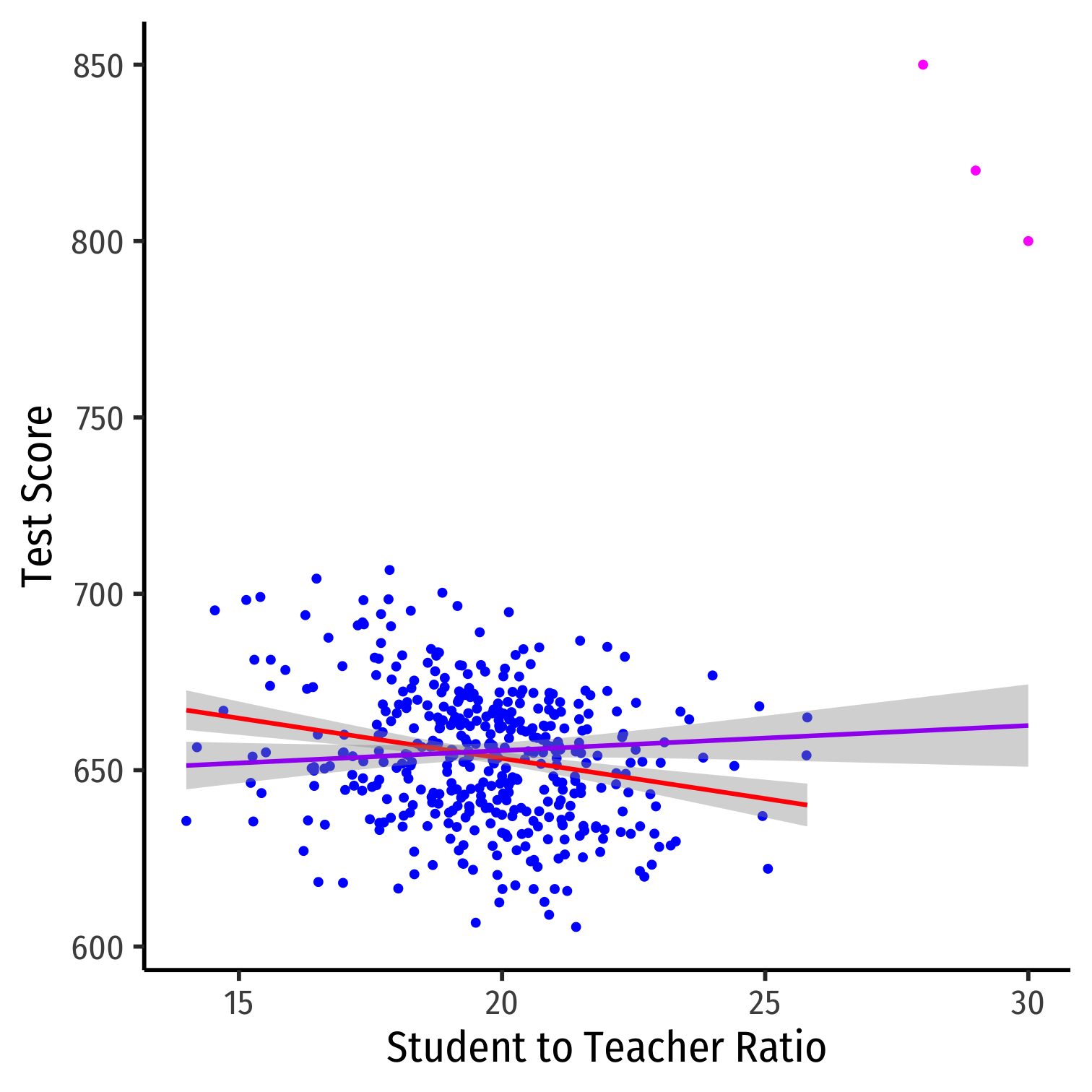
Outliers Can Bias OLS! I
Outliers can affect the slope (and intercept) of the line and add bias
- May be result of human error (measurement, transcribing, etc)
- May be meaningful and accurate
In any case, compare how including/dropping outliers affects regression and always discuss outliers!