Bivariate Data: Scatterplots
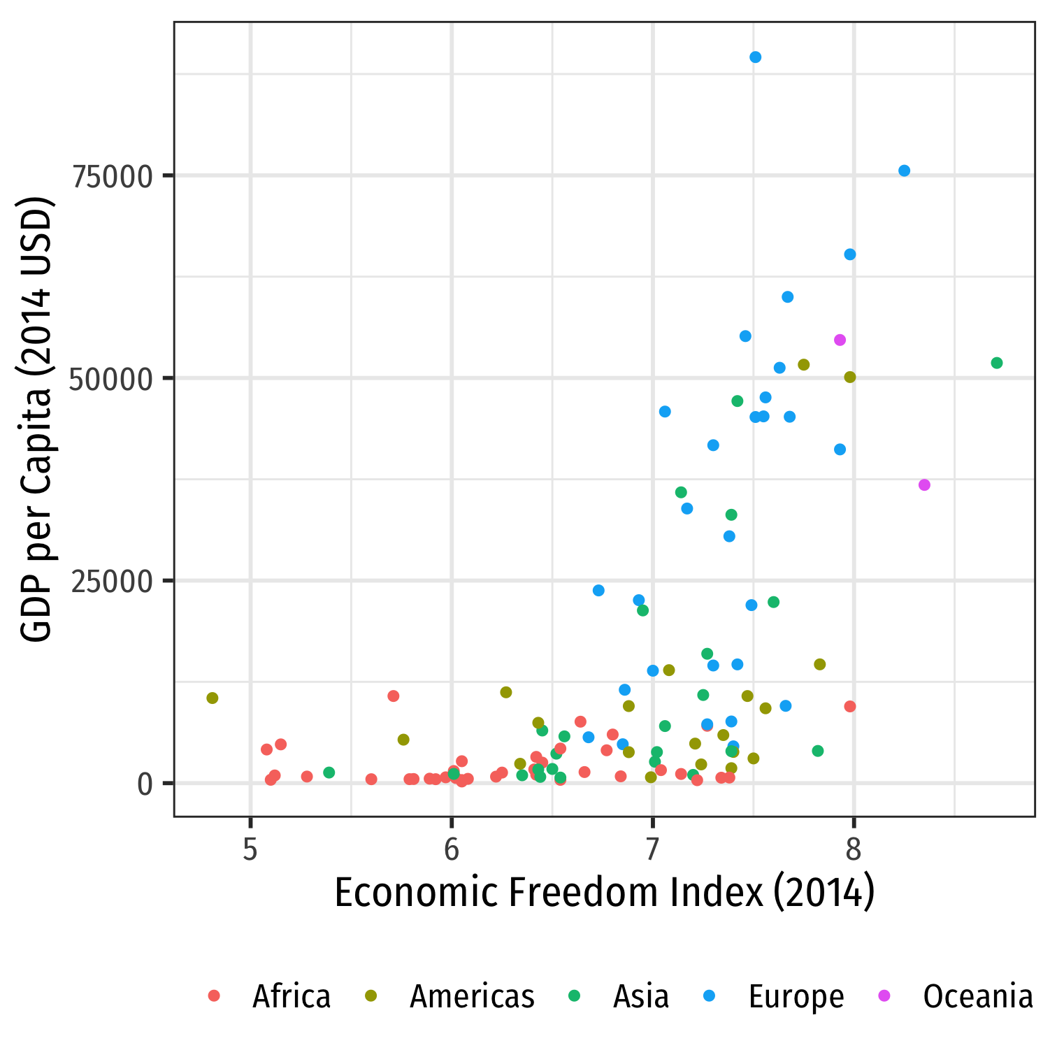
The best way to visualize an association between two variables is with a scatterplot
Each point: pair of variable values (xi,yi)∈X,Y for observation i
library("ggplot2")ggplot(data = econfreedom)+ aes(x = ef, y = gdp)+ geom_point(aes(color = continent), size = 2)+ labs(x = "Economic Freedom Index (2014)", y = "GDP per Capita (2014 USD)", color = "")+ theme_bw(base_family = "Fira Sans Condensed", base_size=20)+ theme(legend.position = "bottom")
Associations
- Look for association between independent and dependent variables
Direction: is the trend positive or negative?
Form: is the trend linear, quadratic, something else, or no pattern?
Strength: is the association strong or weak?
Outliers: do any observations break the trends above?
Correlation: Interpretation
- Correlation is standardized to
−1≤r≤1
- Negative values ⟹ negative association
- Positive values ⟹ positive association
- Correlation of 0 ⟹ no association
- As |r|→1⟹ the stronger the association
- Correlation of |r|=1⟹ perfectly linear
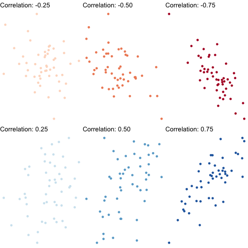
Guess the Correlation!

Correlation and Covariance in R II
corrplot(gapminder_cor_table, type="upper", method = "circle", # number for showing correlation coefficient order="alphabet", col=brewer.pal(n=8, name="RdBu"))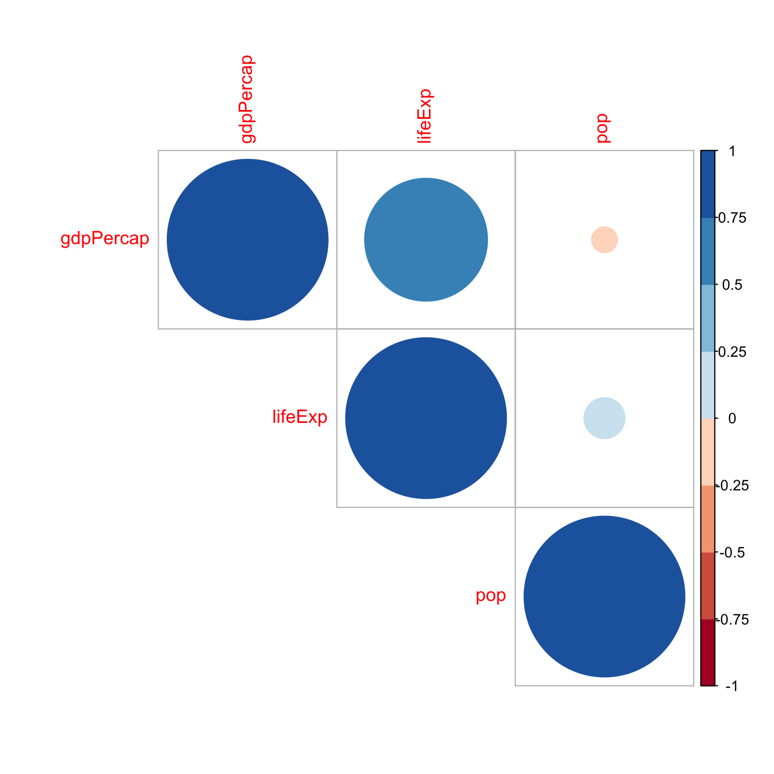
Correlation and Endogeneity
Your Occasional Reminder: Correlation does not imply causation!
- I'll show you the difference in a few weeks (when we can actually talk about causation)
If X and Y are strongly correlated, X can still be endogenous!
See today's class notes page for more on Covariance and Correlation

Always Plot Your Data!

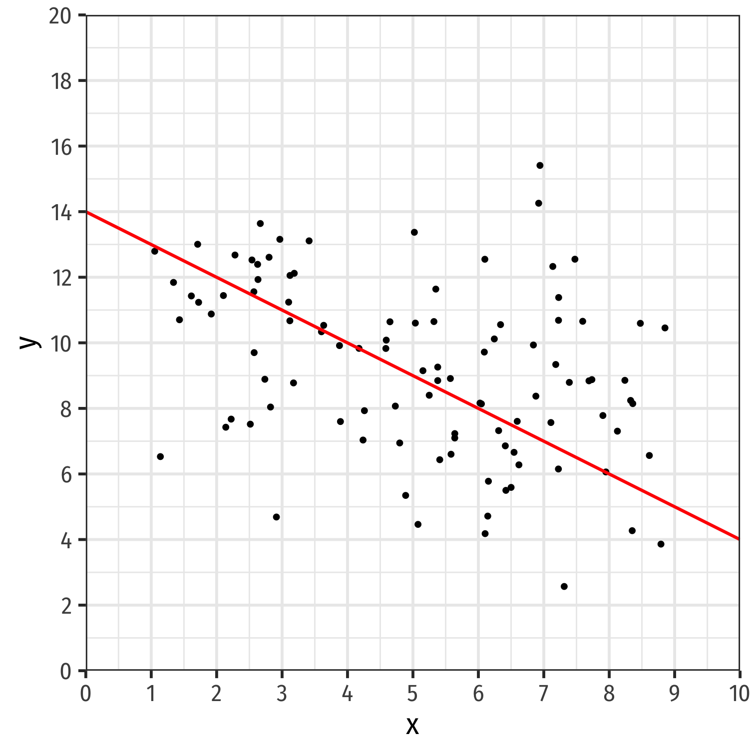
Fitting a Line to Data
- If an association appears linear, we can estimate the equation of a line that would "fit" the data
Y=a+bX
- Recall a linear equation describing a line contains:1
- a: vertical intercept
- b: slope
1 Note we'll use different symbols for a & b, the standard econometric notation.
Fitting a Line to Data
- If an association appears linear, we can estimate the equation of a line that would "fit" the data
Y=a+bX
Recall a linear equation describing a line contains:1
- a: vertical intercept
- b: slope
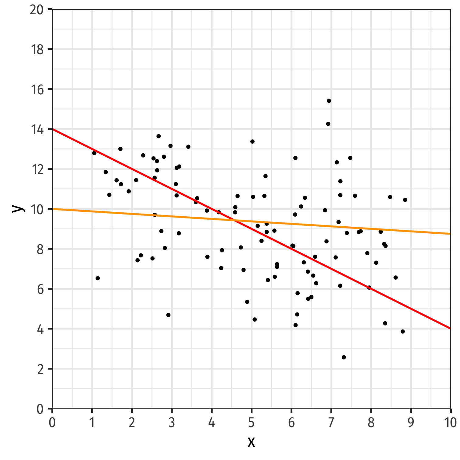
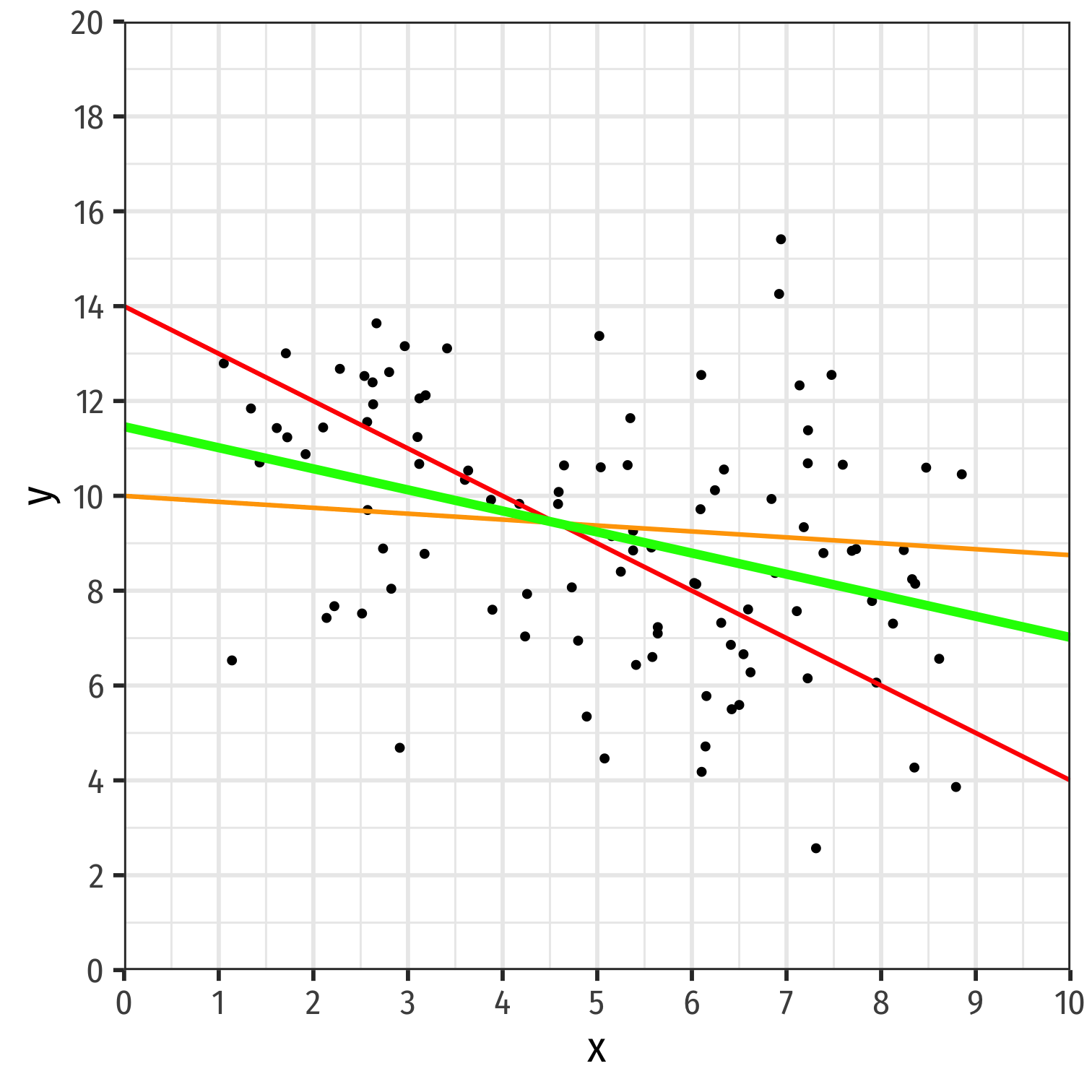
How do we choose the equation that best fits the data?
1 Note we'll use different symbols for a & b, the standard econometric notation.
Fitting a Line to Data
- If an association appears linear, we can estimate the equation of a line that would "fit" the data
Y=a+bX
Recall a linear equation describing a line contains:1
- a: vertical intercept
- b: slope
How do we choose the equation that best fits the data?
This process is called linear regression
1 Note we'll use different symbols for a & b, the standard econometric notation.
Class Size Example
Example: What is the relationship between class size and educational performance?

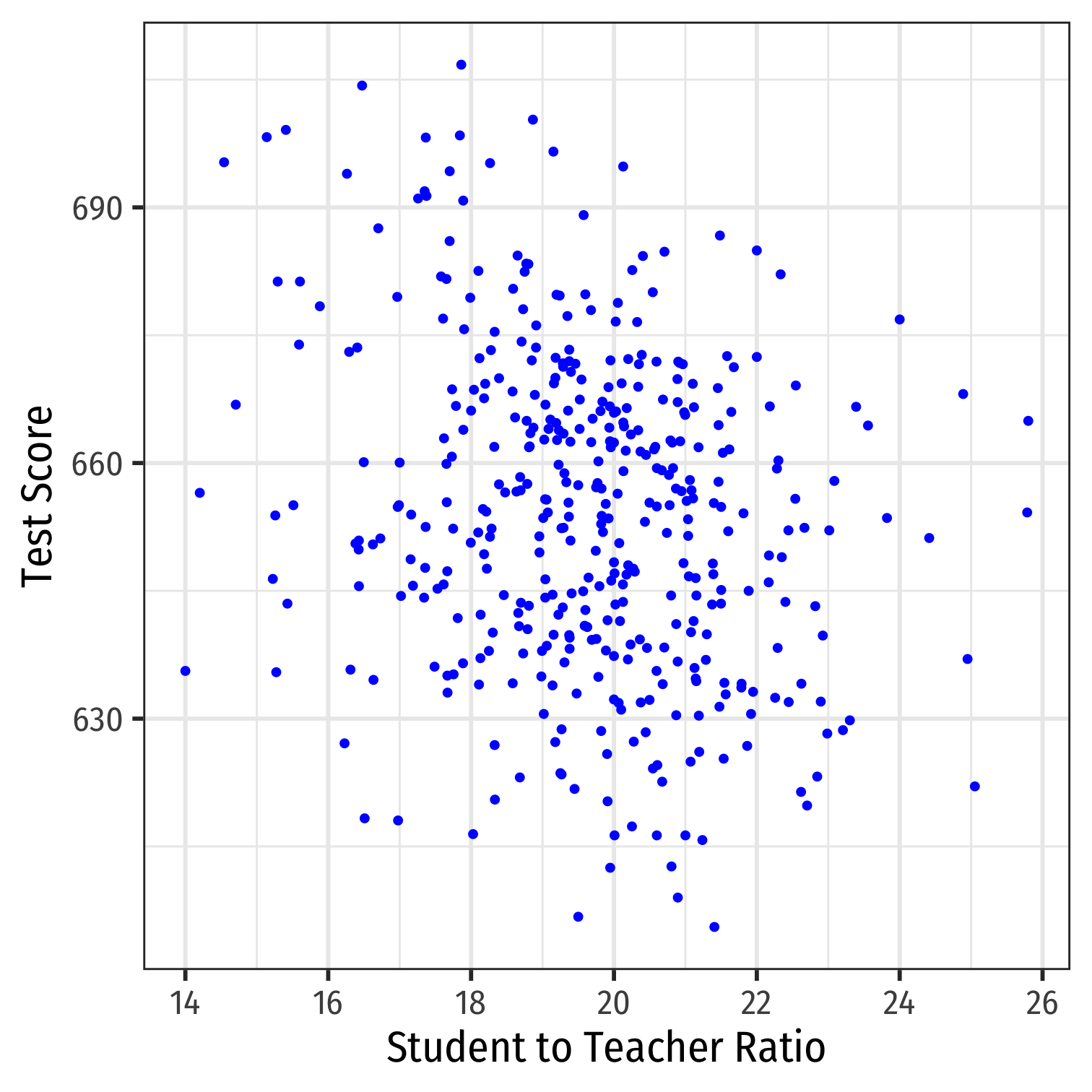
Class Size Example: Scatterplot
scatter<-ggplot(data = CASchool)+ aes(x = str, y = testscr)+ geom_point(color = "blue")+ labs(x = "Student to Teacher Ratio", y = "Test Score")+ theme_bw(base_family = "Fira Sans Condensed", base_size = 20)scatter
Class Size Example: Slope I
- If we change (Δ) the class size by an amount, what would we expect the change in test scores to be?
β=change in test scorechange in class size=Δtest scoreΔclass size
- If we knew β, we could say that changing class size by 1 student will change test scores by β
Class Size Example: Slope II
- Rearranging:
Δtest score=β×Δclass size
Class Size Example: Slope II
- Rearranging:
Δtest score=β×Δclass size
- Suppose β=−0.6. If we shrank class size by 2 students, our model predicts:
Δtest score=−2×βΔtest score=−2×−0.6Δtest score=1.2
Class Size Example: Slope and Average Effect
test score=β0+β1×class size
The line relating class size and test scores has the above equation
β0 is the vertical-intercept, test score where class size is 0
β1 is the slope of the regression line
This relationship only holds on average for all districts in the population, individual districts are also affected by other factors
Class Size Example: Marginal Effects
- To get an equation that holds for each district, we need to include other factors
test score=β0+β1class size+other factors
For now, we will ignore these until Unit 3
Thus, β0+β1class size gives the average effect of class sizes on scores
Later, we will want to estimate the marginal effect (causal effect) of each factor on an individual district's test score, holding all other factors constant
The Population Regression Model
How do we draw a line through the scatterplot? We do not know the "true" β0 or β1
We do have data from a sample of class sizes and test scores1
So the real question is, how can we estimate β0 and β1?
1 Data are student-teacher-ratio and average test scores on Stanford 9 Achievement Test for 5th grade students for 420 K-6 and K-8 school districts in California in 1999, (Stock and Watson, 2015: p. 141)

Deriving OLS
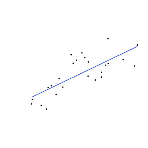
- Suppose we have some data points
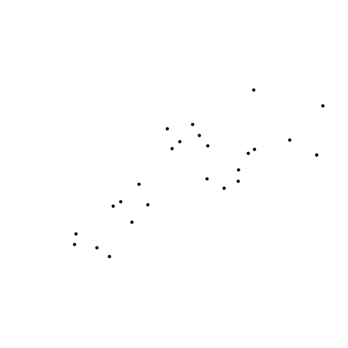
Deriving OLS
- Suppose we have some data points
- We add a line
Deriving OLS
- Suppose we have some data points
- We add a line
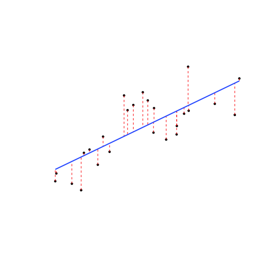
- The residual, ˆu of each data point is the difference between the actual and the predicted value of Y given X:
ui=Yi−^Yi
Deriving OLS
- Suppose we have some data points
- We add a line
- The residual, ˆu of each data point is the difference between the actual and the predicted value of Y given X:
ui=Yi−^Yi
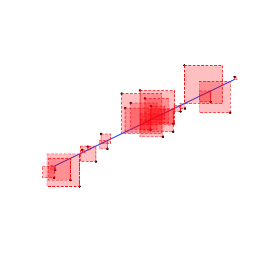
- We square each residual

Deriving OLS
- Suppose we have some data points
- We add a line
- The residual, ˆu of each data point is the difference between the actual and the predicted value of Y given X:
ui=Yi−^Yi
- We square each residual
- Add all of these up: Sum of Squared Errors (SSE)
SSE=n∑i=1u2i
Deriving OLS
- Suppose we have some data points
- We add a line
- The residual, ˆu of each data point is the difference between the actual and the predicted value of Y given X:
ui=Yi−^Yi
- We square each residual
- Add all of these up: Sum of Squared Errors (SSE)
SSE=n∑i=1u2i
- The line of best fit minimizes SSE

Class Size Scatterplot (Again)
scatterThere is some true (unknown) population relationship: test score=β0+β1×str
β1=Δtest scoreΔstr=??
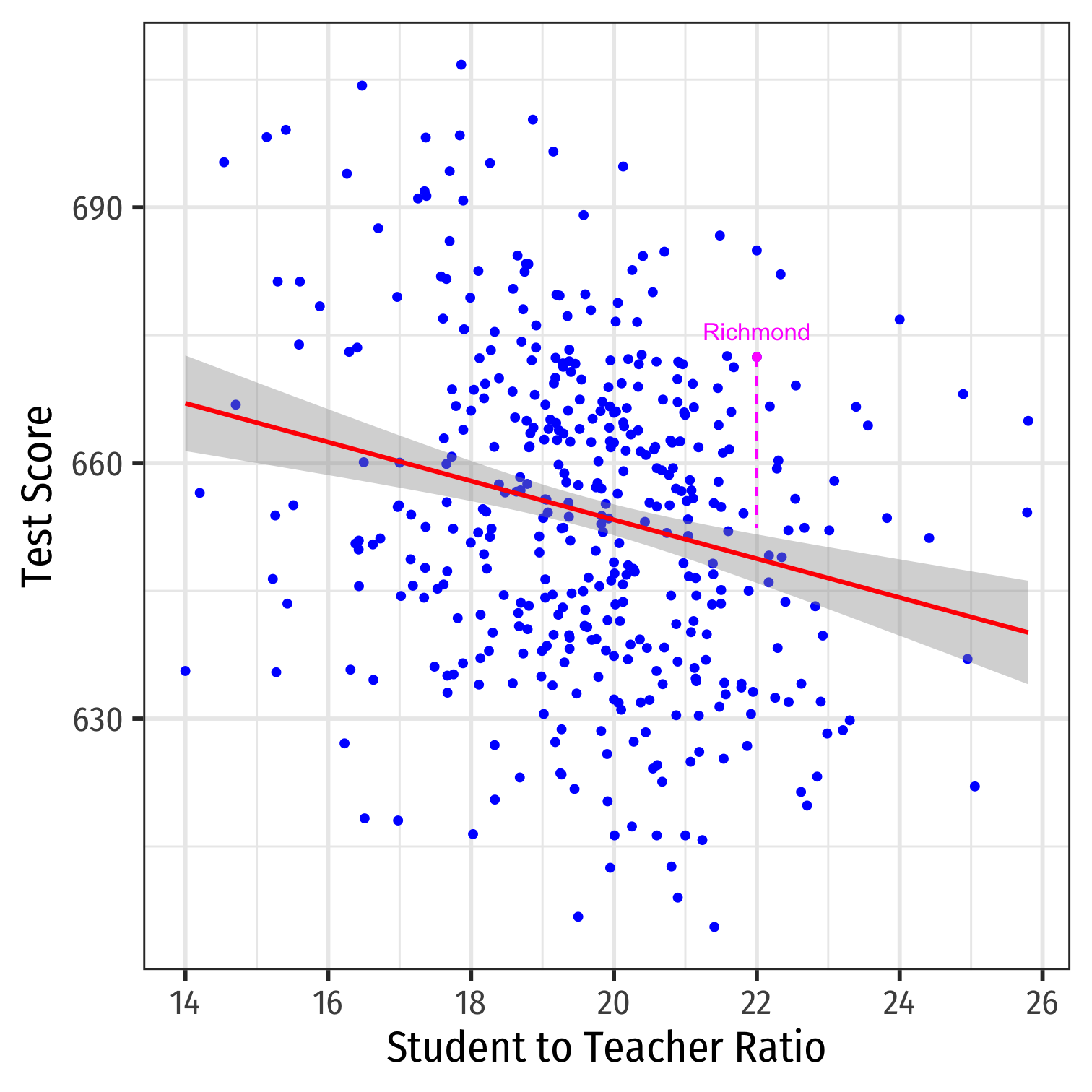
Class SIze Scatterplot with Regression Line
scatter+ geom_smooth(method = "lm", color = "red")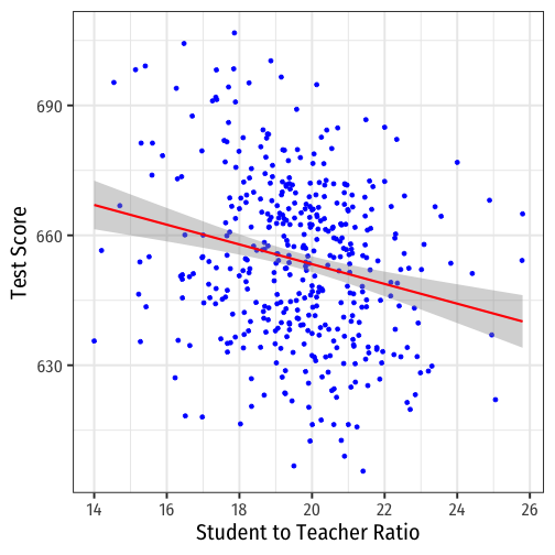
Tidy OLS in R: broom I

The
broompackage allows us to tidy up regression objects1The
tidy()function creates a tidytibbleof regression output
# load packageslibrary(broom)# tidy regression outputtidy(school_reg)## # A tibble: 2 x 5## term estimate std.error statistic p.value## <chr> <dbl> <dbl> <dbl> <dbl>## 1 (Intercept) 699. 9.47 73.8 6.57e-242## 2 str -2.28 0.480 -4.75 2.78e- 61 See more at broom.tidyverse.org.
Tidy OLS in R: broom II
The
broompackage allows us to tidy up regression objects1The
tidy()function creates a tidytibbleof regression output
# load packageslibrary(broom)# tidy regression output (with confidence intervals!)tidy(school_reg, conf.int = TRUE)## # A tibble: 2 x 7## term estimate std.error statistic p.value conf.low conf.high## <chr> <dbl> <dbl> <dbl> <dbl> <dbl> <dbl>## 1 (Intercept) 699. 9.47 73.8 6.57e-242 680. 718. ## 2 str -2.28 0.480 -4.75 2.78e- 6 -3.22 -1.341 See more at broom.tidyverse.org.
Class Size Regression: A Data Point
- One district in our sample is Richmond, CA:
CASchool %>% filter(district=="Richmond Elementary") %>% dplyr::select(district, testscr, str)## # A tibble: 1 x 3## district testscr str## <chr> <dbl> <dbl>## 1 Richmond Elementary 672. 22Predicted value: ^Test ScoreRichmond=698−2.28(22)≈648
Residual: ˆuRichmond=672−648≈24