Two Big Problems with Data
- We want to use econometrics to identify causal relationships and make inferences about them
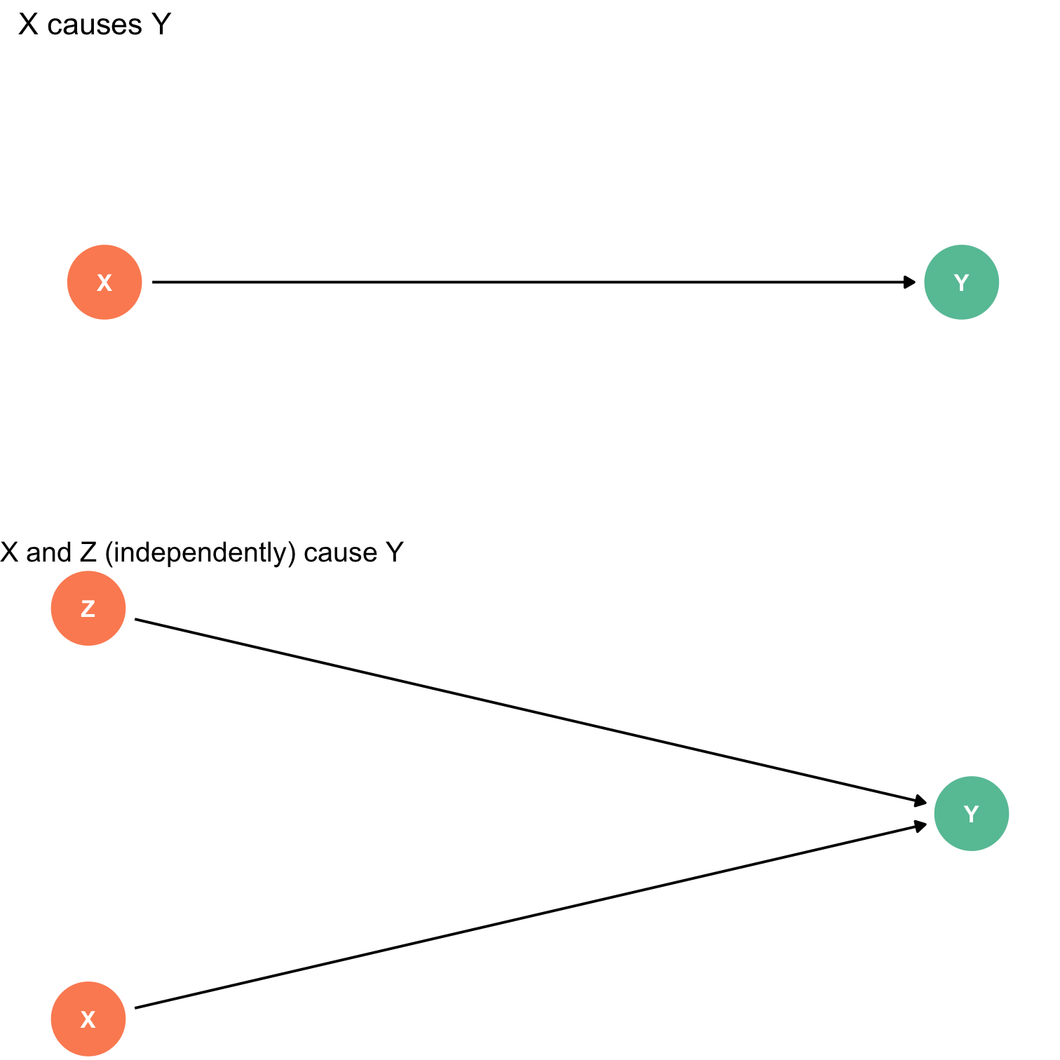
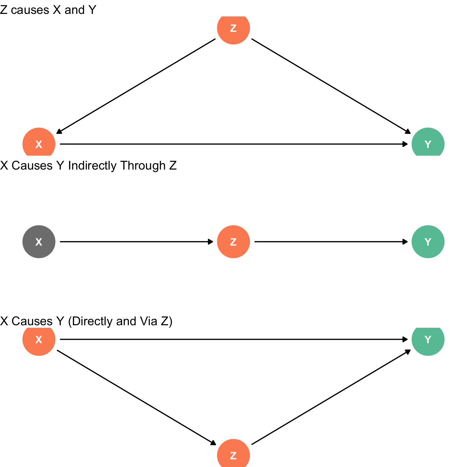
Problem for identification: endogeneity
Problem for inference: randomness

Identification Problem: Endogeneity I
An independent variable (X) is exogenous if its variation is unrelated to other factors that affect the dependent variable (Y)
An independent variable (X) is endogenous if its variation is related to other factors that affect the dependent variable (Y)

Identification Problem: Endogeneity II
- An independent variable (X) is exogenous if its variation is unrelated to other factors that affect the dependent variable (Y)
Identification Problem: Endogeneity III
- An independent variable (X) is endogenous if its variation is related to other factors that affect the dependent variable (Y)
Identification Problem: Endogeneity IV
Confusingly, these terms mean something different in econometrics than in the theoretical economics models where you have heard them before
In Theoretical models:
- "Exogenous": a parameter determined outside of the model and taken as given
- "Endogenous": a variable whose value is determined by the model

Identification Problem: Endogeneity V
Example 1: In a classic supply and demand model:
- Exogenous parameters: income, prices of other goods, cost, technology
- Endogenous variables: equilibrium price, equilibrium quantity
Identification Problem: Endogeneity VI
Example 2: In a consumer optimization model:
- Exogenous parameters: market prices, income, utility function
- Endogenous variables: utility-maximizing bundle of goods
Inference Problem: Randomness
Data is random due to natural sampling variation
- Taking one sample of a population will yield slightly different information than another sample of the same population
Common in statistics, easy to fix
Inferential Statistics: making claims about a wider population using sample data
- We use common tools and techniques to deal with randomness

Random Controlled Trials (RCTs) I
- The ideal way to demonstrate causation is through a randomized controlled trial (RCT) or "random experiment"
- Randomly assign experimental units (e.g. people, firms, etc.) into groups
- Treatment group(s) get a (kind of) treatment
- Control group gets no treatment
- Compare results of treatment and control groups to observe the average treatment effect (ATE)
- We will understand "causality" to mean the ATE from an ideal RCT

Random Controlled Trials (RCTs) II

Classic (simplified) procedure of a randomized control trial (RCT) from medicine
Random Controlled Trials (RCTs) III
- Random assignment to groups ensures that the only differences between members of the treatment(s) and control groups is receiving treatment or not
 Treatment Group
 Control Group
Random Controlled Trials (RCTs) IV
Random assignment to groups ensures that the only differences between members of the treatment(s) and control groups is receiving treatment or not
Selection bias: (pre-existing) differences between members of treatment and control groups other than treatment, that affect the outcome
Treatment Group
Control Group
(Selection Bias)
Example: The Effect of Having Health Insurance I
Example: What is the effect of having health insurance on health outcomes?
National Health Interview Survey (NHIS) asks "Would you say your health in general is excellent, very good, good, fair, or poor?"
Outcome variable (Y): Index of health (1-poor to 5-excellent) in a sample of married NHIS respondents in 2009 who may or may not have health insurance
Treatment (X): Having health insurance (vs. not)

Example: The Effect of Having Health Insurance II

Angrist, Joshua & Jorn-Steffen Pischke, 2015, Mostly Harmless Econometrics
Example: A Hypothetical Comparison
| John | Maria |
|---|---|
 |
 |
| Y0J=3 | Y0M=5 |
| Y1J=4 | Y1M=5 |
Example: A Hypothetical Comparison
| John | Maria |
|---|---|
|
|
| Y0J=3 | Y0M=5 |
| Y1J=4 | Y1M=5 |
John will choose to buy health insurance
Maria will choose to not buy health insurance
Example: A Hypothetical Comparison
| John | Maria |
|---|---|
|
|
| Y0J=3 | Y0M=5 |
| Y1J=4 | Y1M=5 |
| Y1J−Y0J=1 | Y1M−Y0M=0 |
John will choose to buy health insurance
Maria will choose to not buy health insurance
Health insurance improves John's score by 1, has no effect on Maria's score
Example: A Hypothetical Comparison
| John | Maria |
|---|---|
|
|
| Y0J=3 | Y0M=5 |
| Y1J=4 | Y1M=5 |
| Y1J−Y0J=1 | Y1M−Y0M=0 |
| YJ=(Y1J)=4 | YM=(Y0M)=5 |
John will choose to buy health insurance
Maria will choose to not buy health insurance
Health insurance improves John's score by 1, has no effect on Maria's score
Note, all we can observe in the data are their health outcomes after they have chosen (not) to buy health insurance: YJ=4 and YM=5
Observed difference between John and Maria: YJ−YM=−1
Counterfactuals
| John | Maria |
|---|---|
|
|
| YJ=4 | YM=5 |
This is all the data we actually observe
Observed difference between John and Maria: YJ−YM=Y1J−Y0M⏟=−1
Recall:
- John has bought health insurance (Y1J)
- Maria has not bought insurance (Y0M)
We don't see the counterfactuals:
- John's score without insurance
- Maria score with insurance
Counterfactuals
| John | Maria |
|---|---|
|
|
| YJ=4 | YM=5 |
This is all the data we actually observe
Observed difference between John and Maria: YJ−YM=Y1J−Y0M⏟=−1
Algebra trick: add and subtract Y0J to equation
Yj−YM=Y1J−Y0J⏟=1+Y0J−Y0M⏟=−2
- Y1J−Y0J=1: Causal effect for John of buying insurance
- Y0J−Y0M=−2: Difference between John & Maria pre-treatment, "selection bias"
Example II
Y0J−Y0M≠0
- Selection bias: (pre-existing) differences between members of treatment and control groups other than treatment, that affect the outcome
- i.e. John and Maria start out with very different health scores before either decides to buy insurance or not ("recieve treatment" or not)
John (Treated)
Maria (Control)
Random Assignment: The Silver Bullet
If treatment is randomly assigned for a large sample, it eliminates selection bias!
Treatment and control groups differ on average by nothing except treatment status
Creates ceterus paribus conditions in economics: groups are identical on average (holding constant age, sex, height, etc.)
Treatment Group
Control Group
The Quest for Causal Effects I
RCTs are considered the "gold standard" for causal claims
But society is not our laboratory (probably a good thing!)
We can rarely conduct experiments to get data

The Quest for Causal Effects II
Instead, we often rely on observational data
This data is not random!
Must take extra care in forming an identification strategy
To make good claims about causation in society, we must get clever!

Natural Experiments
Economists often resort to searching for natural experiments
Some events beyond our control occur that separate otherwise similar entities into a "treatment" group and a "control" group that we can compare
e.g. natural disasters, U.S. State laws, military draft

The First Natural Experiment

Jon Snow
The First Natural Experiment

1813-1858
John Snow utilized the first famous natural experiment to establish the foundations of epidemiology and the germ theory of disease
Water pumps with sources downstream of a sewage dump in the Thames river spread cholera while water pumps with sources upstream did not

For the Next Few Classes
